What is the first step of getting your hands dirty?
Table 1:Iris dataset.
| ID | Variety | Sepal Length | Sepal Width | Petal Length | Petal Width |
|---|---|---|---|---|---|
| 0 | Setosa | 5.1 | 3.5 | 1.4 | 0.2 |
| 1 | Setosa | 4.9 | 3 | 1.4 | 0.2 |
| 2 | Setosa | 4.7 | 3.2 | 1.3 | 0.2 |
| 3 | Setosa | 4.6 | 3.1 | 1.5 | 0.2 |
| 4 | Setosa | 5 | 3.6 | 1.4 | 0.2 |
| .. | ... | ... | ... | ... | ... |
First Step: Draw the frequency distribution.
Below is an example of Iris’ petal length from week 1, when we talked about the analysis of differences.
The frequency distributions were drawn separately for different species of Iris, which provided a visual comparison between the three species.
Are them different?
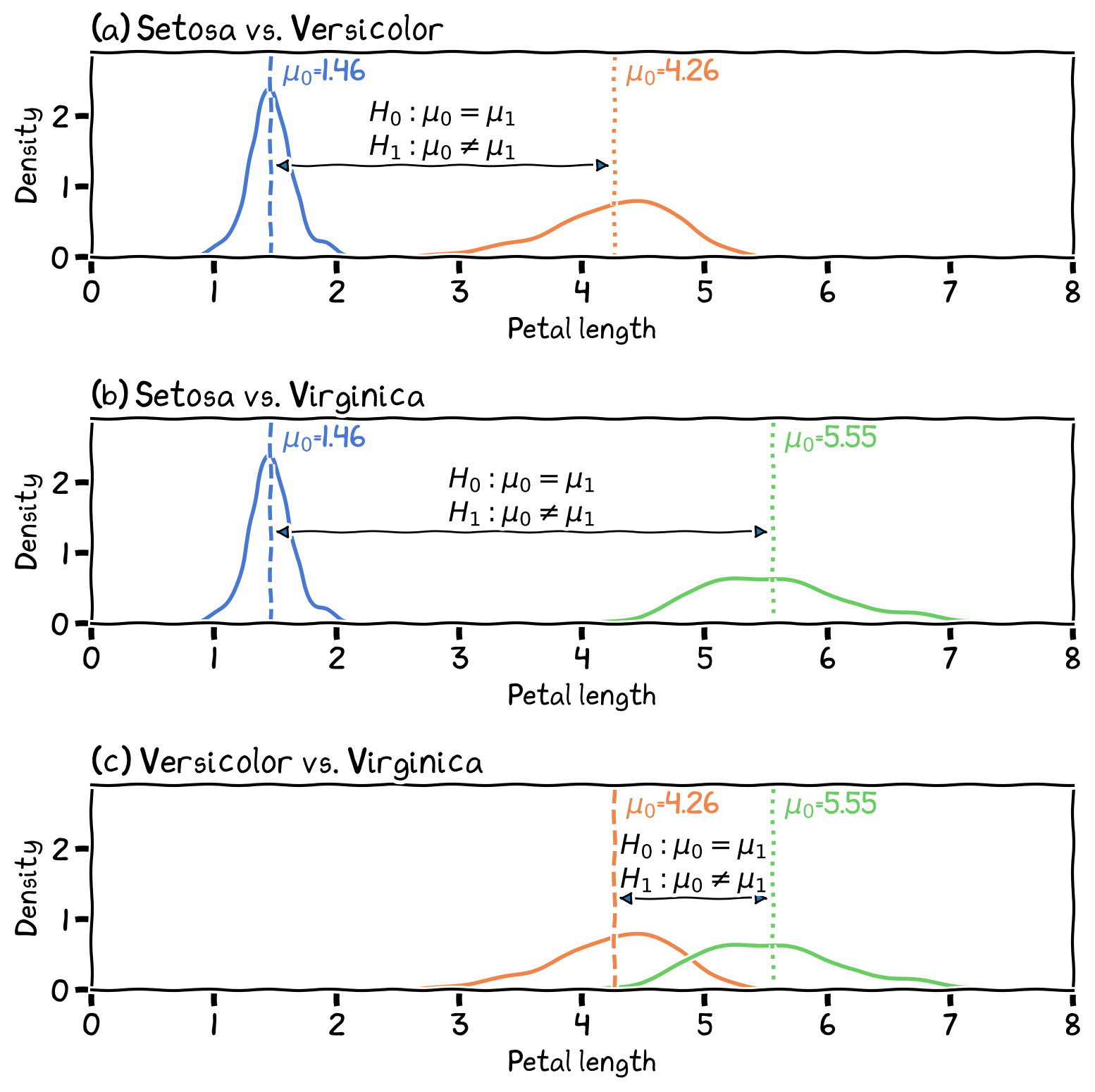
The differences in petal length between the three species.
Define Differences
In statistics, “difference” typically refers to the extent to which two or more groups, samples, or observations differ from one another. This can be quantified and assessed through various statistical measures and analyses, depending on the nature of the data and research questions.
Groups: by genders, by years, by types
Data point in groups: individual participant, transaction, bus stop, district

How to determine if they are different or not so different?
Spotting The Differences
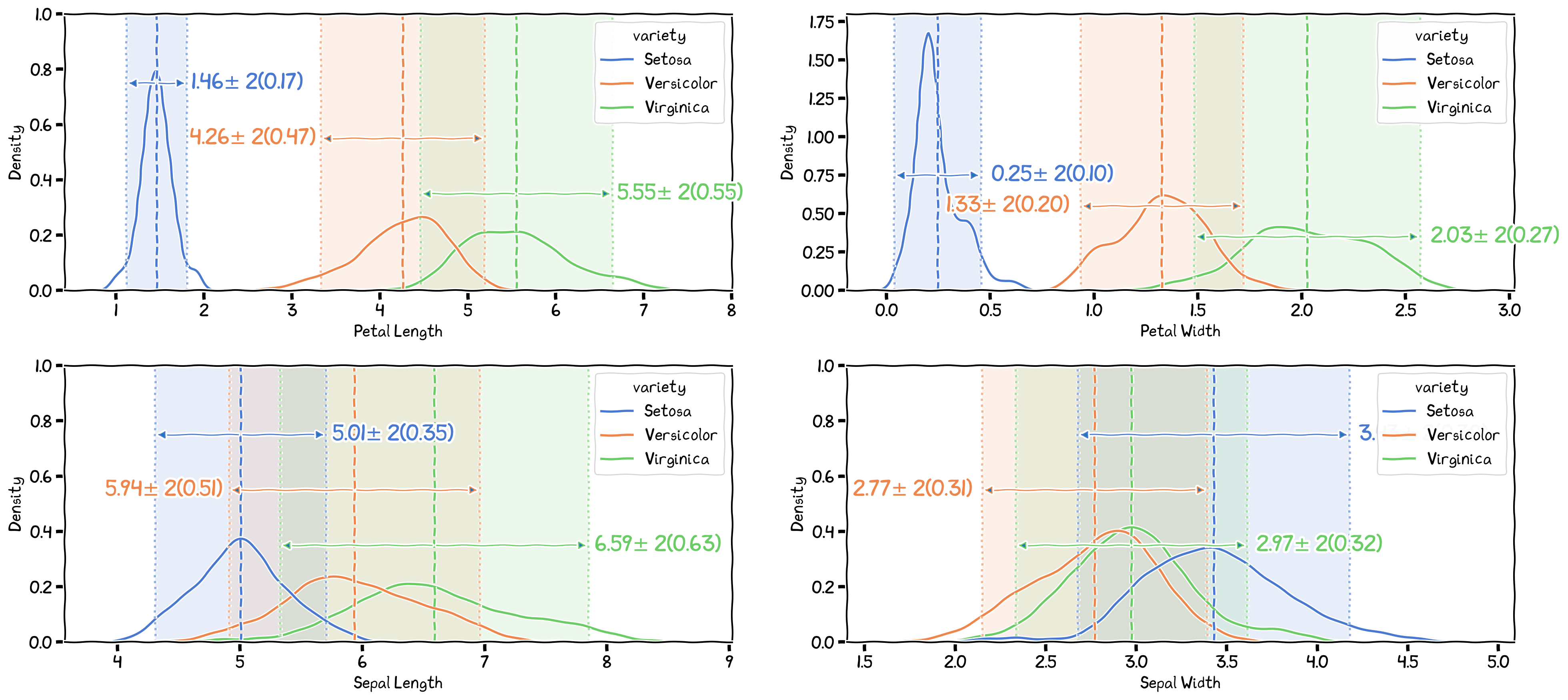
The differences in the 4 variables between species.
Hypothesis Testing
Hypothesis testing is a statistical method used to evaluate claims or assertions about a population parameter by analyzing sample data.
The goal is to determine if the observed differences between groups or samples are statistically significant or merely due to chance.
What does it means by ‘due to chance’?
In another chapter, we talked about Normal Distribution, and why ‘Normal’ is ‘Normal’.
When we get a set of samples, the samples’ distribution tend to form a bell-shape, i.e., high at the middle (the central tendency), and dropped from middle to both sides (the spread). But why?
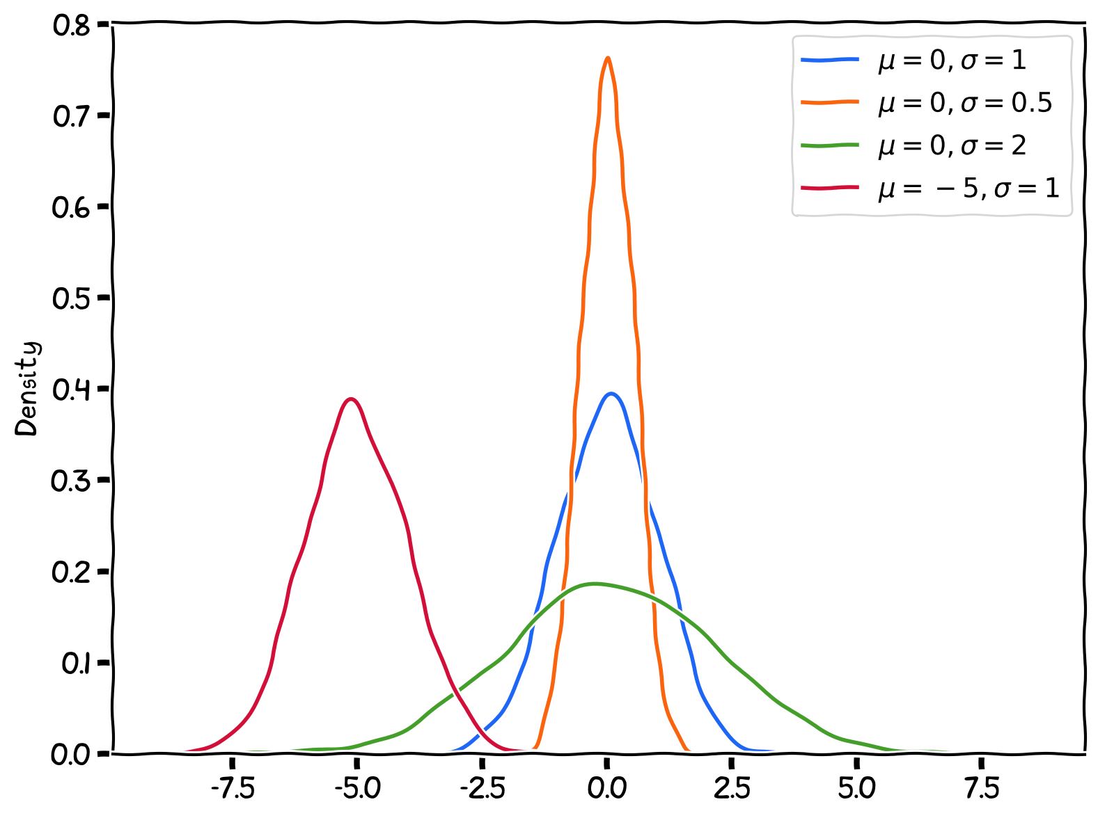
The Normal Distribution.
The variance, or spread, of a dataset can result from various factors, including random processes, natural variation, or systematic differences. Despite this variability, data points often cluster around a central value due to underlying patterns or tendencies within the population.
In other words, values that fall at positive or negative distances from the mean may be influenced by random factors or chance. This also applies when we draw a value and obtain an extreme value far from the center---such values can occur due to randomness or chance.
Everything can happen by chance---so when we see one value that is away from the sample mean, it does not promise to be ‘different’ from the distribution.

Figure 5:A data point compared to the distribution.
Let’s say we have a class of students, and their height values are measured and which shows a normal distribution (Figure 5), i.e., mean=170, std=10.
At this point, you can view these students as a set of sample, sampling from the population (the university). The university’s students height should (or can be assumed to) form a normal distribution.
Now, you get a student from the next door, and his height is 135. Deos it means this person is different from the currect class?
Strategy for measuring difference of an individual data point from a distribution
Calculate how far this data point is from the average of the distribution.
How many standard deviation it is from the distribution’s mean? (the z-score that use mean and std)
How many deviance (MAD) it is from the distribution’s median? (use median and MAD)
Comparison of two distributions
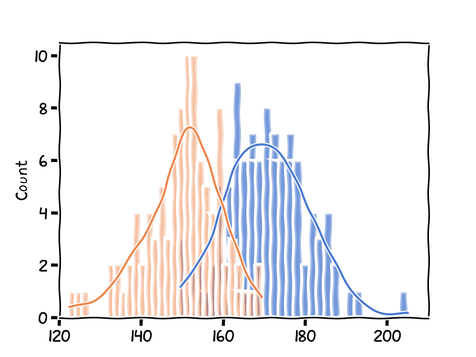
The distributions of two groups of students.
Next, get a series of students’ height from next door, perhaps the same number of students as the first class and which generate a distribution (another normal distribution).
Then, how to compare them?
Central values and spread Central values can be represented by measures of central tendency, such as the mean, median, or mode. In many situations, particularly when data follow a normal distribution, the combination of central tendency and spread can provide a helpful summary of the overall distribution and its characteristics.
Shape and other measurements Assume to be normal distribution
Strategy for comparison
Compare the mean between the two distributions
Compare the spread of the two distributions
Key Concepts
Hypothesis testing is a crucial tool in statistical inference and helps researchers make data-driven decisions about the relationships or differences between variables.
Null Hypothesis ():
A statement that assumes no significant difference between the variables.
The goal of hypothesis testing is to gather evidence to reject the null hypothesis.
Essentially, the null hypothesis reflects the idea of “no effect” or “no difference.”
Alternative Hypothesis ( or ):
A statement that assumes a significant difference between the variables.
This is the hypothesis we aim to support when rejecting the null hypothesis.
The alternative hypothesis is basically about “has effect” or “has difference.”
Test Statistic:
A value calculated from the sample data to assess the likelihood of obtaining the observed results under the assumption that the null hypothesis is true.
Depending on the assumptions that fit the situation, the tests for assessing the differences are T-test, ANOVA, and their non-parametric alternatives.
Significance Level ():
The threshold probability for rejecting the null hypothesis, often set at 0.05 or 0.01.
It represents the probability threshold of incorrectly rejecting the null hypothesis when it is true (Type I error). (The risk that we are willing to take.)
p-value:
The probability of obtaining the observed results (or more extreme results) under the assumption that the null hypothesis is true.
A small p-value indicates that the observed results are unlikely to occur by chance alone, providing evidence to reject the null hypothesis.
The risk of being wrong to reject
Statistical Significance:
When the p-value is less than the chosen significance level (), we reject the null hypothesis and conclude that the results are statistically significant, supporting the alternative hypothesis ().
Otherwise, we fail to reject it.
About Type 1 and Type 2 errors
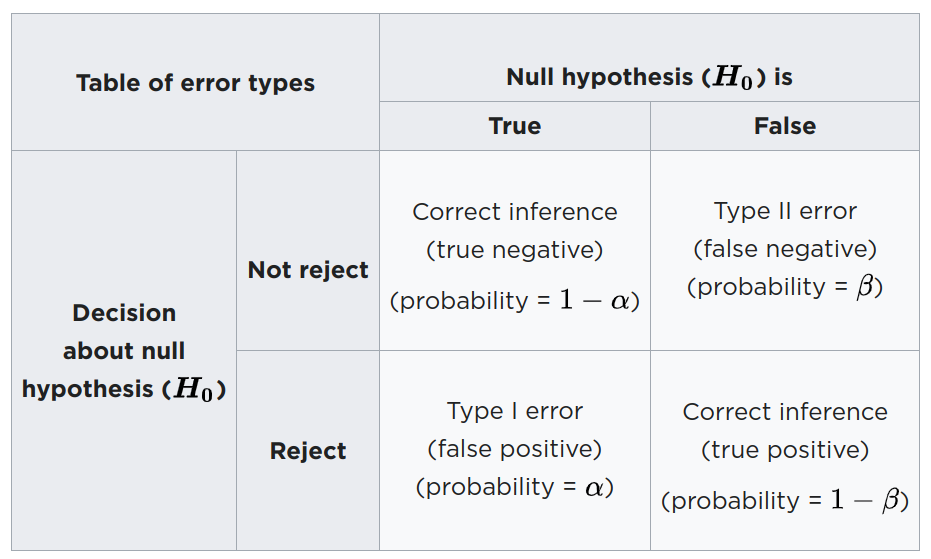
Type 1 and type 2 errors. Table from Wikipedia
Hypothesis for Testing the Differences
The null hypothesis reflects the idea of “no effect” or “no difference.”
Hypothesis for testing differences between two means:
Hypothesis for testing differences between more than two means:
Null hypothesis is something that we DO NOT NEED to prove, because it cannot be proven anyway.
The null hypothesis is assumed to be true until the data provide sufficient evidence against it.
We can only gather evidence to reject the null hypothesis, not to confirm or prove it.
Failing to reject the null hypothesis doesn’t necessarily mean it’s true; it simply indicates that there’s insufficient evidence to support the alternative hypothesis.
For Spatial Patterns Detection
Is the spatial pattern different from a random pattern?
null hypothesis: no difference
Is there any significant clusters?
null hypothesis: no clustering effect