Assumptions of t-tests
To ensure the validity of the results, the t-test relies on certain assumptions:
.bold[Continuous]: The data (target variable) should be continuous (interval/ratio).
.bold[Normality]: The data should be approximately normally distributed.
.bold[Independence]: Observations .red[within and between groups] should be independent (not influence one another).
.bold[Homogeneity of variances]: The variances (or standard deviations) of the groups should be approximately equal (this assumption can be relaxed for some t-tests).
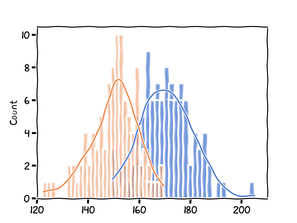
The distributions of two groups of students.
Two Types of ‘Groups’: Between vs. Within
‘Between’-Group Analysis
Number of subject groups: 2 or more
Number of target variables: 1 (for every subject)
Purpose: To compare differences among distinct groups of subjects.
‘Within’-Group Analysis
Number subject groups: 1
Number of target variables: 2 or more (for every subject)
Purpose: To examine the differences or changes within a single group over time or under different conditions.
Types of t-tests
There are three main types of t-tests:
One sample t-test
Independent samples t-test
Paired samples t-test
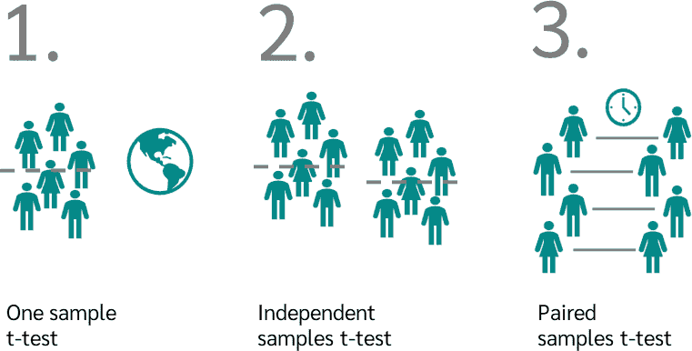
Source: Datatab
One sample t-test
Compares the mean of a single group to a known population mean.
E.g., the students’ performances from one school compared to the national mean; the air polution level compared to the safety standards...
Each individual or observation in the sample contributes to a single group being compared to the known population mean.
Source: Datatab
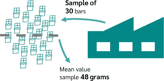
An example
A factory claims that their light bulbs have an average lifespan of hours. A consumer group selects a random sample of 25 bulbs and finds that the sample has an average lifespan of 985 hours with a standard deviation of 50 hours. The consumer group wants to determine whether the factory’s claim is accurate.
[ 935,  969,  917,  922,  906, 1022,  984, 1023, 1042,  944,
  982, 1054,  923, 1012,  963, 1011,  924, 1026, 1081,  932,
 1027,  947,  994, 1016, 1069 ]
The one sample t-test example.
.bold[Finding]: The consumer group cannot conclude that the factory’s claim is inaccurate based on this sample. There is not enough evidence to reject the null hypothesis that the average lifespan of the light bulbs is 1,000 hours.
Steps involved in the one-sample t-test:
Formulate the null hypothesis () and the alternative hypothesis ():
: The average lifespan of the light bulbs is 1,000 hours (.
: The average lifespan of the light bulbs is not 1,000 hours ().
Calculate the t-test statistic (t) using the formula:
t = (sample mean - population mean) / (standard error of the mean)
standard error of the mean
Plugging in the values:
Determine the degrees of freedom (df), which is equal to
the sample size minus 1 (df = n - 1);
.
Using the t-value (-1.5) and degrees of freedom (24), find the p-value associated with the test statistic from the t-distribution table or by using statistical software:
The p-value is approximately 0.16.
Since the p-value (0.16) is greater than the conventional significance level of 0.05, we fail to reject the null hypothesis.
Independent samples t-test
Compares the means of two independent groups.
E.g., the scores of students from two classes; the effect of treatment vs. placebo-control groups...
Every individual will only appear in only one of the two groups.

Source: Datatab
In each subplot, the mean of two Iris species were compared.
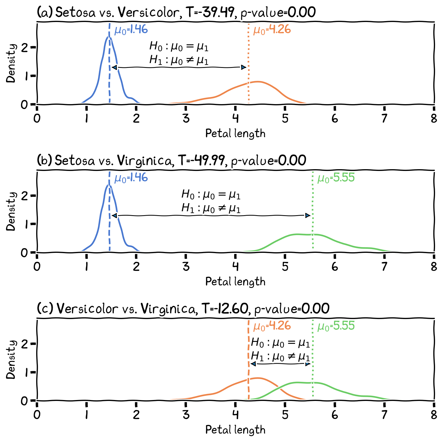
The differences in petal length between the three species, with t-test results.
Paired samples t-test
Compares the means of two related or paired groups.
E.g., pre-test and post-test scores from the same group of individuals; differences between spouses or siblings...
Every individual in the pre-test group must also be present in the post-test group, or each individual in one group should have a specific counterpart in the other group.

Source: Datatab
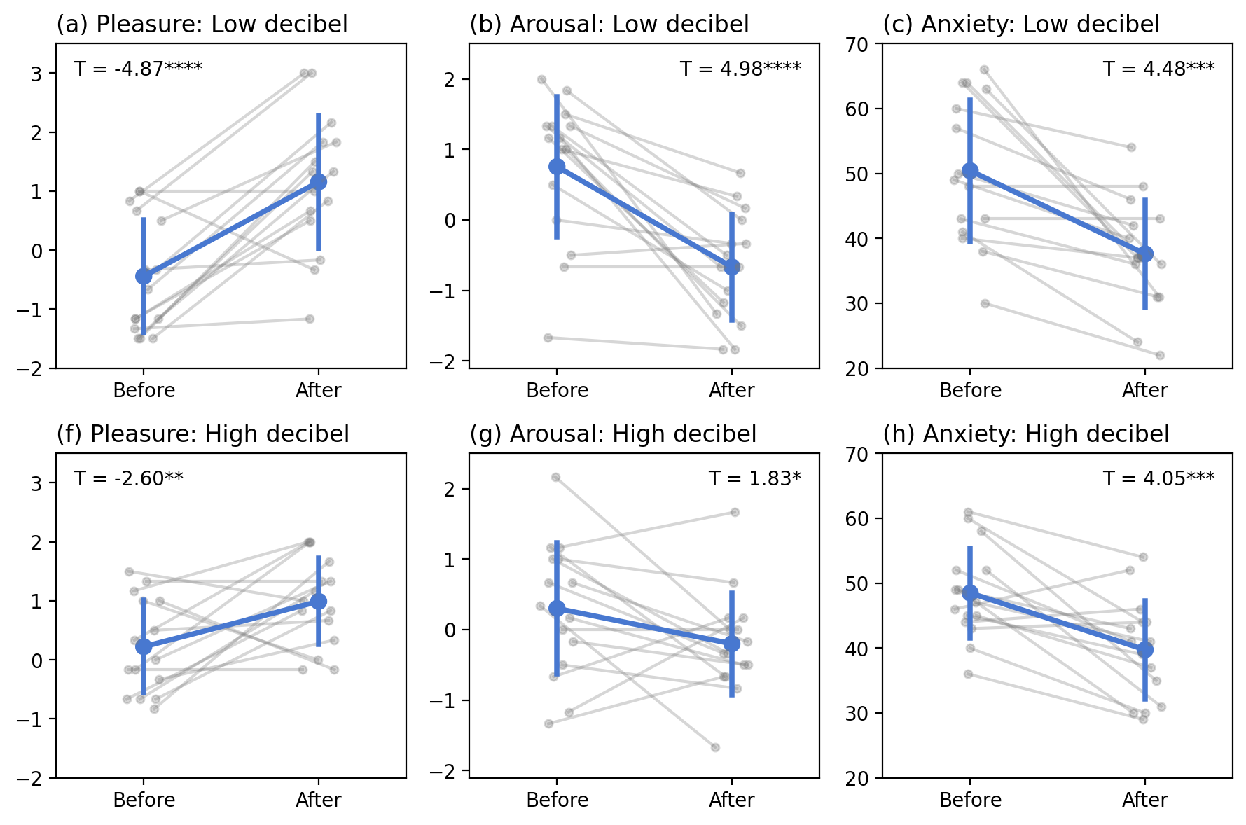
The changes of psychological indexes before and after a VR treatment. T-test and significant levels are shown at top right. Hsieh et al. (2023)
T-Test Statistic and Interpretation
t-value (aka T-statistic)
The t-test calculates a t-value by dividing the difference between the group means by the standard error of the difference. A higher t-value (positive or negative) suggests a larger inter-group difference relative to the intra-group variability.
p-value
The t-test also provides a p-value, which represents the probability of observing a t-value at least as extreme as the one calculated, assuming the null hypothesis is true. A lower p-value indicates stronger evidence against the null hypothesis, suggesting a significant difference between the groups.
Degrees of Freedom
Degrees of freedom (df) are used to determine the appropriate t-distribution for calculating p-values. For independent samples t-test, , where and are the sample sizes of the two groups.
Effect Size
To assess the practical significance of the difference between group means, effect size measures like Cohen’s d, Eta-squared, and Hedge’s g can be calculated. Cohen’s d indicates the magnitude of the difference between the groups in standard deviation units.
Cohen’s d: Cohen’s d is a standardized measure of effect size, often used in comparing the means of two groups. It expresses the difference between group means in terms of standard deviations, making it a useful metric for comparing effects across different studies. The guidelines proposed by Jacob Cohen for interpreting d are:
Small effect: d = 0.2
Medium effect: d = 0.5
Large effect: d = 0.8
Eta-squared (η²): Eta-squared is often reported in the context of ANOVA (Analysis of Variance) tests. It describes the proportion of variance in the dependent variable that can be explained by the independent variable. Eta-squared values range from 0 to 1, with higher values indicating larger effects. Here are some general guidelines for interpreting η²:
Small effect: η² = 0.01
Medium effect: η² = 0.06
Large effect: η² = 0.14
Hedge’s g: Hedge’s g, like Cohen’s d, is a standardized effect size measure for comparing two group means. However, it includes a correction for bias in small samples, making it more appropriate than Cohen’s d when sample sizes are small. The interpretation guidelines for Hedge’s g are similar to Cohen’s d:
Small effect: g = 0.2
Medium effect: g = 0.5
Large effect: g = 0.8
Common Language Effect Size (CLES): The Common Language Effect Size (CLES) is a non-parametric effect size measure that communicates the likelihood that a randomly selected observation from one group will be greater than a randomly selected observation from another group. CLES offers a more intuitive understanding of statistical results, making it easier for researchers and non-experts to interpret the practical significance of findings.
Summary
The t-test is widely used in various fields to compare group means and evaluate the effectiveness of treatments, interventions, or different conditions. It serves as an essential tool for hypothesis testing and data analysis.
- Hsieh, C.-H., Yang, J.-Y., Huang, C.-W., & Chin, W. C. B. (2023). The effect of water sound level in virtual reality: A study of restorative benefits in young adults through immersive natural environments. Journal of Environmental Psychology, 88, 102012. 10.1016/j.jenvp.2023.102012