The conceptual definition
Kernel Density Estimation (KDE) is a non-parametric technique for estimating the probability density function---the kernel function---of a continuous variable. KDE is widely used in various fields, such as statistical analysis, machine learning, and data visualization. The main idea behind KDE is to represent the underlying probability distribution of a dataset by summing up the influence of individual data points.
Key properties
Non-parametric approach: KDE does not assume a specific underlying distribution for the data, making it suitable for various types of data distributions.
Smoothing technique: KDE applies a kernel function (e.g., a Gaussian or Epanechnikov kernel) to smooth the input data, resulting in a continuous density estimate.
Bandwidth selection: A crucial aspect of KDE is choosing an appropriate bandwidth or smoothing parameter, which controls the degree of smoothing applied to the data. Optimal bandwidth selection methods, such as cross-validation or plug-in methods, help to balance bias and variance in the density estimate.
Multivariate extension: KDE can be extended to handle multivariate (multi-dimensions) data, providing a way to visualize and analyze the relationships between multiple variables in a dataset.
Probability Density Function
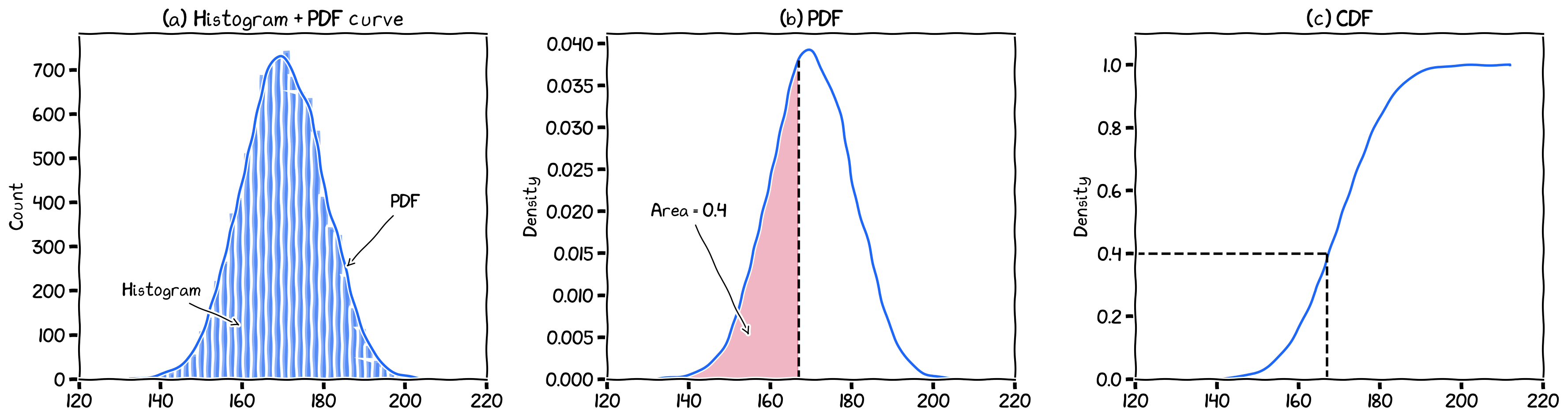
A probability density function (PDF) represents the distribution of a continuous random variable, depicting the likelihood of observing values in a given range.
PDFs provide a comprehensive understanding of the underlying data distribution, including its central tendency, variability, and shape.
They are essential for various data analysis tasks, such as data visualization, outlier detection, and statistical inference.
Remember that we have talked about this in an earlier chapter?
Limitations of Parametric Density Estimation Approaches
Parametric density estimation methods assume that the data follows a specific probability distribution, such as the normal (Gaussian) or exponential distribution.
These methods estimate the distribution parameters (e.g., mean, variance) to characterize the data and make further inferences.
However, the performance of parametric methods heavily relies on the correctness of the assumed distribution, which may not always hold true for real-world datasets.
Incorrect distribution assumptions can lead to biased results and misinterpretations of the data.
The Need for a Flexible and Data-Driven Approach like KDE
KDE is a non-parametric method for estimating probability density functions directly from the data.
KDE does not require strong assumptions about the underlying distribution of the data, making it more flexible and adaptable to various data types and scenarios.
KDE’s data-driven approach allows it to capture complex and irregular features in the data distribution, which may be missed by parametric methods.
By avoiding distribution assumptions, KDE helps mitigate the risk of obtaining misleading results due to incorrect assumptions.
This flexibility and data-driven nature make KDE an attractive choice for a wide range of data analysis tasks, particularly when the underlying distribution is unknown or complex.
In simple words, KDE is a data-driven way to approximate the PDF of data.
Kernel Functions and their properties
A kernel function is a mathematical function used in KDE to assign weights to data points based on their distances from a location of interest.
Kernel functions are characterized by several properties:
Symmetry: The kernel function should be symmetric around the origin, ensuring equal weighting for points equidistant from the location of interest.
Non-negativity: The kernel function should yield non-negative weights, preventing the occurrence of negative density values.
Integration to 1: The kernel function should integrate to 1 over its domain, ensuring that the total density estimated across the entire range of the data sums to 1.
How KDE works
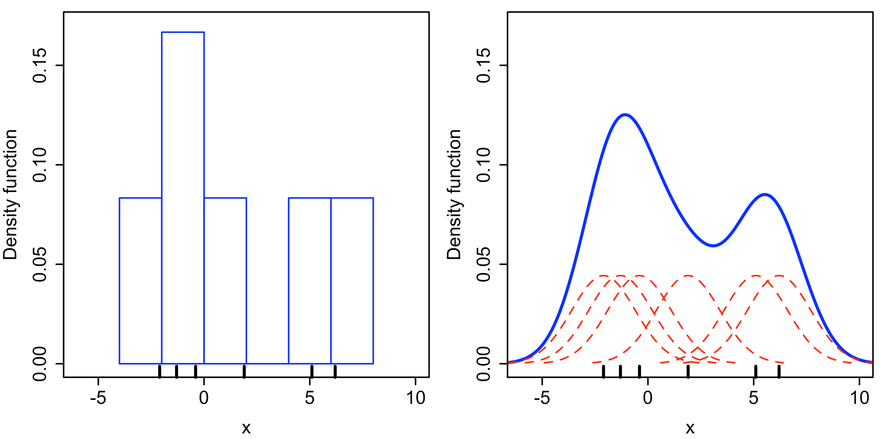
Approach one (from point to space):
For every data point, draw a kernel, i.e., the red dashed lines in left figure.
Stack the kernels if they overlapped, i.e., the blue solid line.
Approach two (from space to point):
For every space unit (x-axis), draw a kernel.
Identify data points that fall within the kernel range.
Measure the distance from data point to the space unit.
Convert the distance to weight using kernel function.
Sum the weight through all identified points in step 2.
A histogram and KDE plot. Image source: Wikipedia
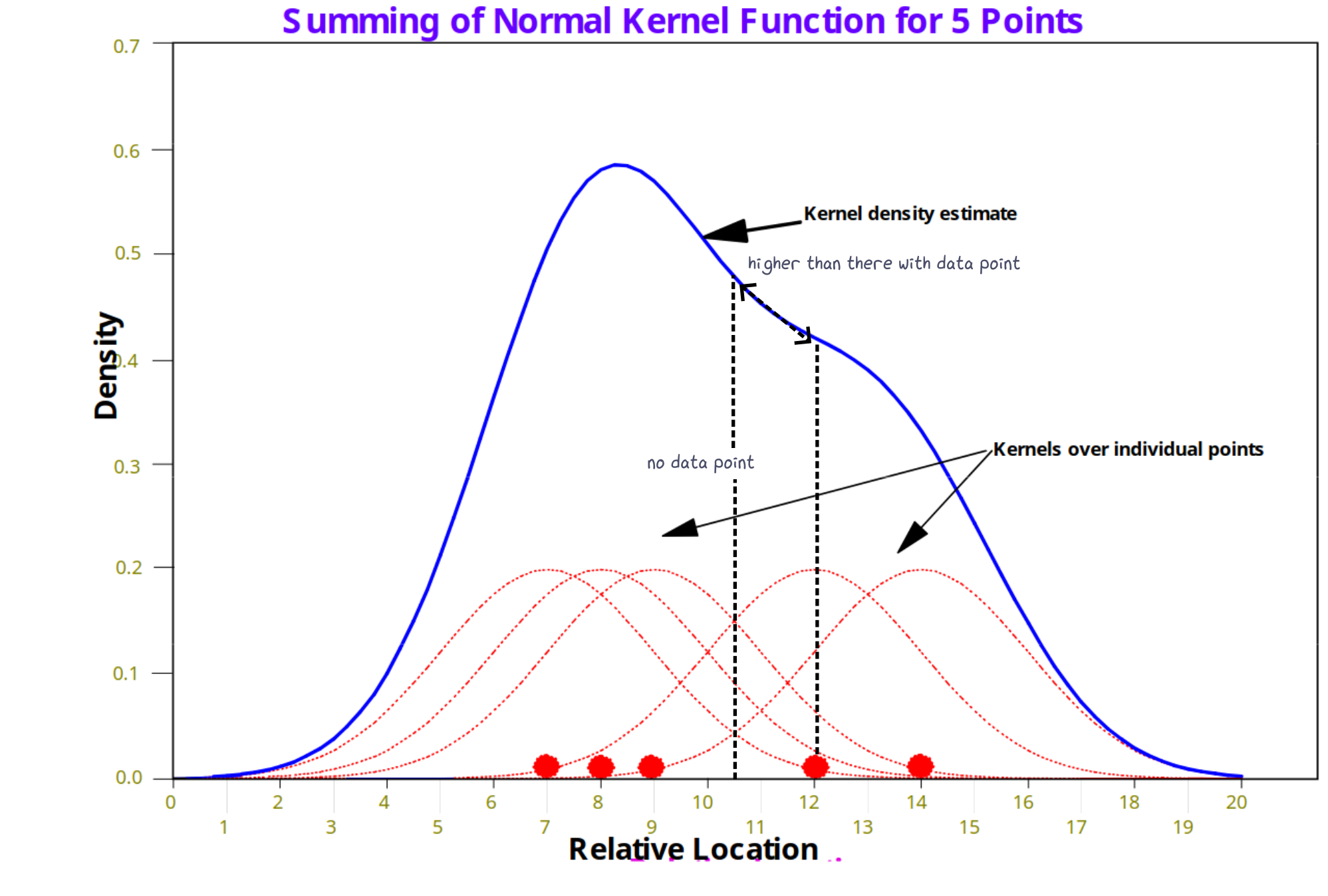
How KDE work: by summing the density value.
Common Kernel Functions
Gaussian kernel
Epanechnikov/Parabolic kernel
Quartic (biweight) kernel
Triangular kernel
Uniform kernel
Gaussian (normal) kernel
The Gaussian kernel follows a bell-shaped curve and is widely used due to its smoothness and differentiability. Its formula is given by:
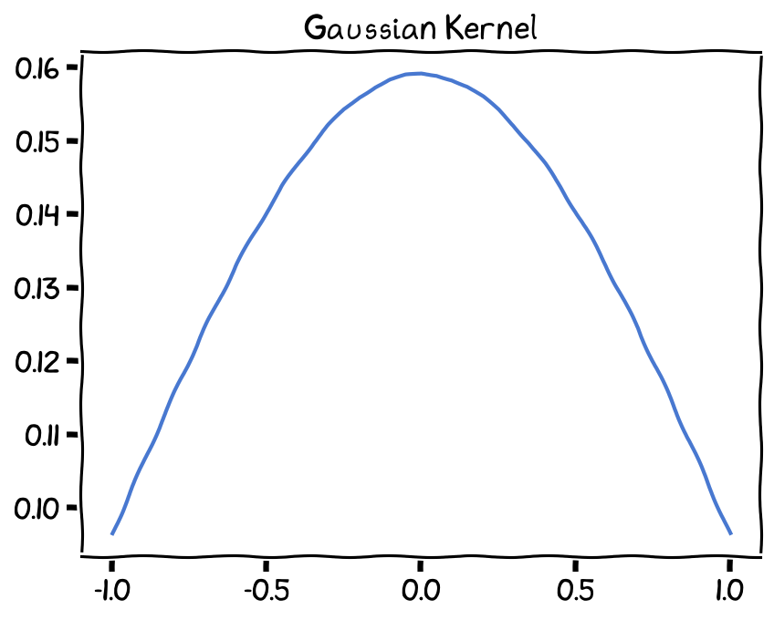
Gaussian Kernel, bandwidth (h) set as 1.
Epanechnikov (parabolic) kernel
The Epanechnikov kernel is optimal for some statistical properties and has a compact support, meaning it assigns zero weight to points outside a specific range. Its formula is:
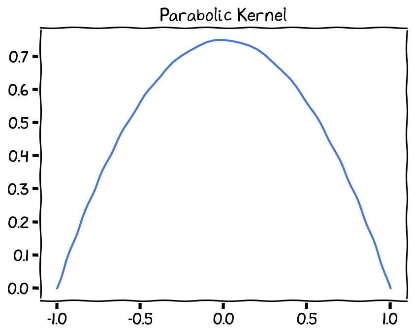
Epanechnikov Kernel, bandwidth (h) set as 1.
Quartic (biweight) kernel
The Quartic kernel function is another commonly used kernel function in Kernel Density Estimation (KDE). It is defined as follows:
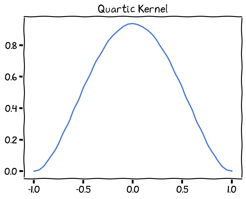
Quartic Kernel, bandwidth (h) set as 1.
Triangular kernel
The Triangular kernel function is a simple and computationally efficient kernel that assigns weights to points based on a triangular shape. It is defined as:
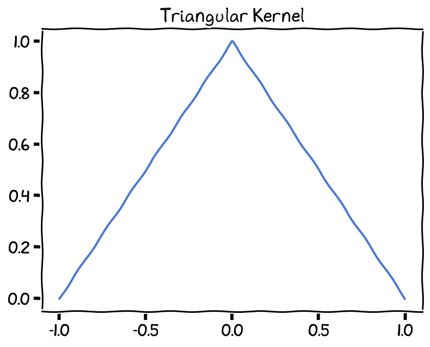
Triangular Kernel, bandwidth (h) set as 1.
Uniform (Tophat) kernel
The uniform kernel assigns equal weights to points within a specific range and zero weight outside that range. Its formula is:
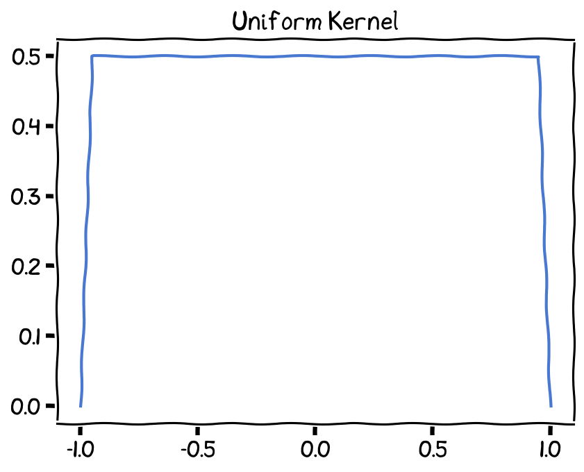
Uniform Kernel, bandwidth (h) set as 1.
The effect of Bandwidth
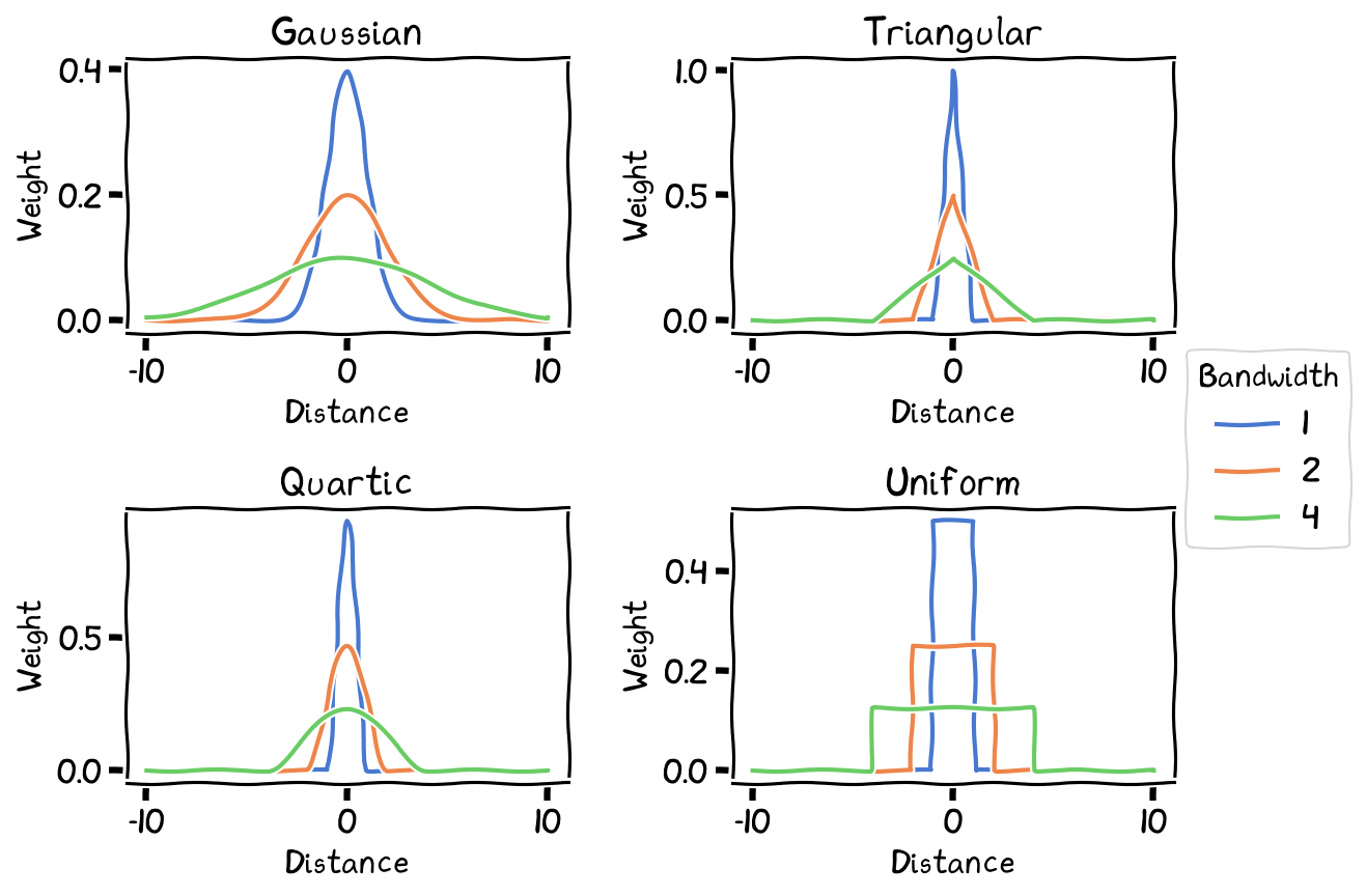
Effect of bandwidth (h) on Kernel Function (weighting).
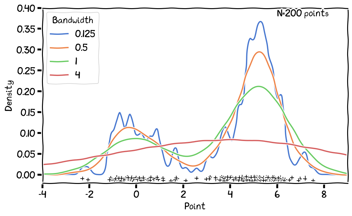
Effect of bandwidth (h) on 1-D KDE results.
Bandwidth Selection
Rule of Thumb
Cross-Validation
Plug-in Methods
Visual Inspection
Rule of Thumb
Silverman’s rule: For a Gaussian kernel,
,
where is the standard deviation of the data, and is the number of data points.
Other heuristics exist for different kernel functions and data dimensions. These rules provide quick estimates but may not be optimal for all datasets.
Cross-Validation
Partition the data into several training sets.
Apply KDE with different bandwidth values to the training set and full dataset.
Calculate the error (MAE, MSE, etc.) between the estimated density and full data set density.
Choose the bandwidth that minimizes the error.
This method is more computationally intensive but provides a more data-driven bandwidth selection.
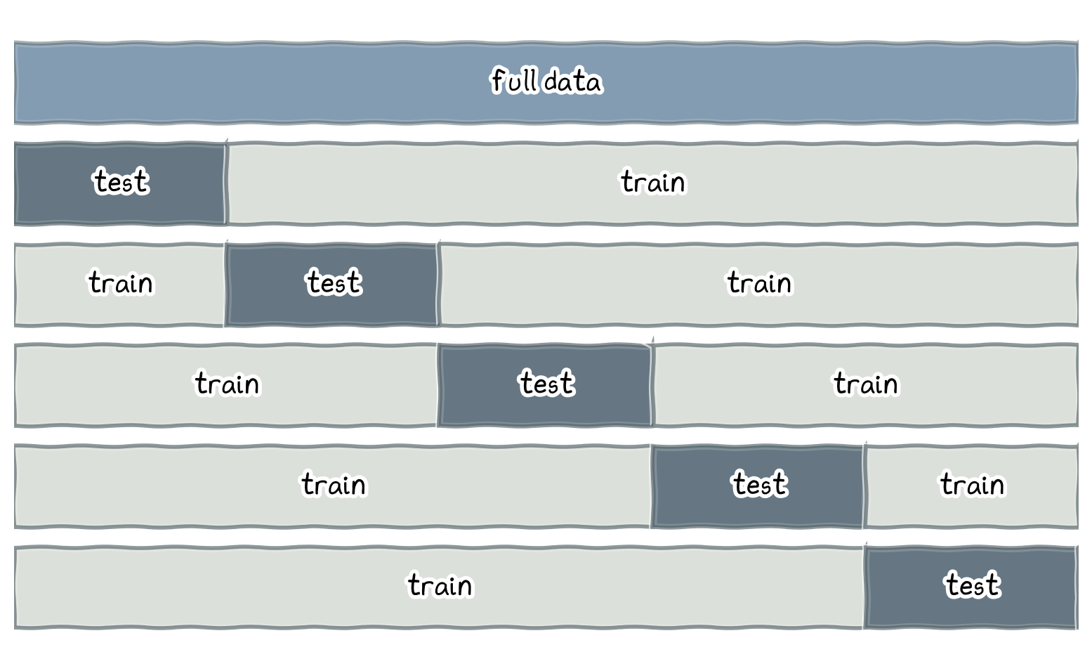
5-fold cross-validation approach.
Plug-in Methods
These methods, such as Least Squares Cross-Validation (LSCV), directly estimate the optimal bandwidth by minimizing an approximation of the Mean Integrated Squared Error (MISE).
Plug-in methods are more complex but can provide better bandwidth estimates in certain scenarios.
Visual Inspection
Plot KDE with different bandwidth values and visually inspect the resulting density estimates.
Choose the bandwidth that produces a density estimate that best captures the underlying structure and trends in the data. This method is subjective and relies on human judgment.
Remarks
In practice, you can start with a rule-of-thumb estimate, then refine it using cross-validation or plug-in methods, and finally perform visual inspection to confirm the selected bandwidth’s appropriateness.
Remember that the best bandwidth may vary depending on the specific data and application.
Advantages of KDE
Non-parametric: Does not assume a specific distribution for the data.
Versatile: Works with various data types and dimensions.
Flexible: Handles complex data structures and multimodal distributions.
Smoothness: Produces smooth, continuous density estimates.
Adaptive: Bandwidth selection allows for control over smoothing.
Intuitive interpretation: Visualization of the density estimate is straightforward.
Wide availability: Implemented in many statistical software packages and libraries.
Disadvantages/ Limitations of KDE
Bandwidth selection: Can be challenging and affect the quality of the density estimate.
Computational complexity: High-dimensional data can make KDE computationally demanding.
Boundary bias: Density estimates can be biased near the boundary of the data.
Curse of dimensionality: Performance deteriorates as the dimension of the data increases.
Sensitivity to outliers: KDE can be influenced by outliers or data sparsity.
Interpretation: Understanding the shape of the density estimate can be subjective.
Lack of model: KDE does not provide a parametric model that can be used for further analysis.
KDE: Visualizing Data Distribution
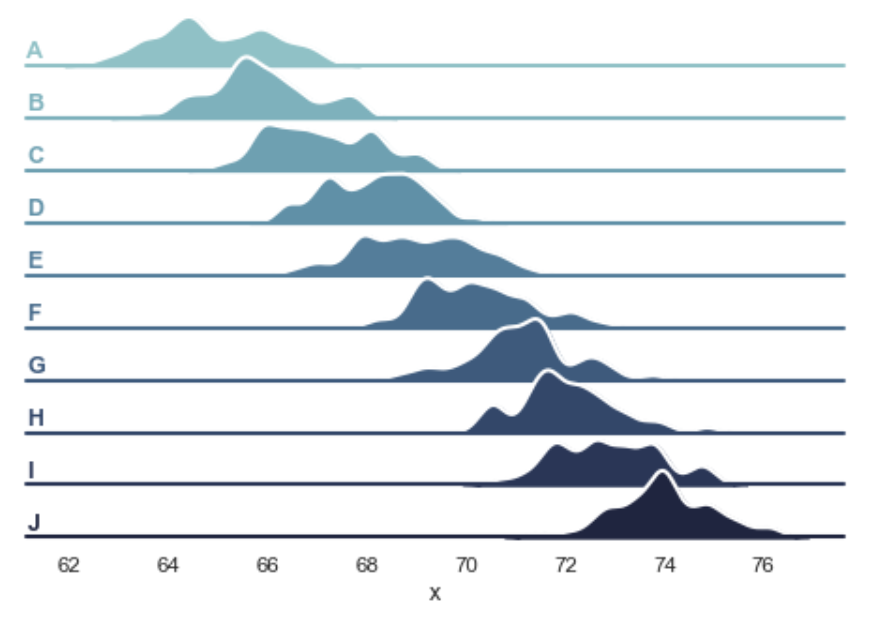
Line fill plot.
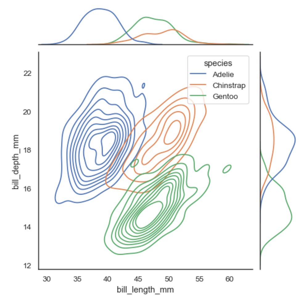
Contour lines.
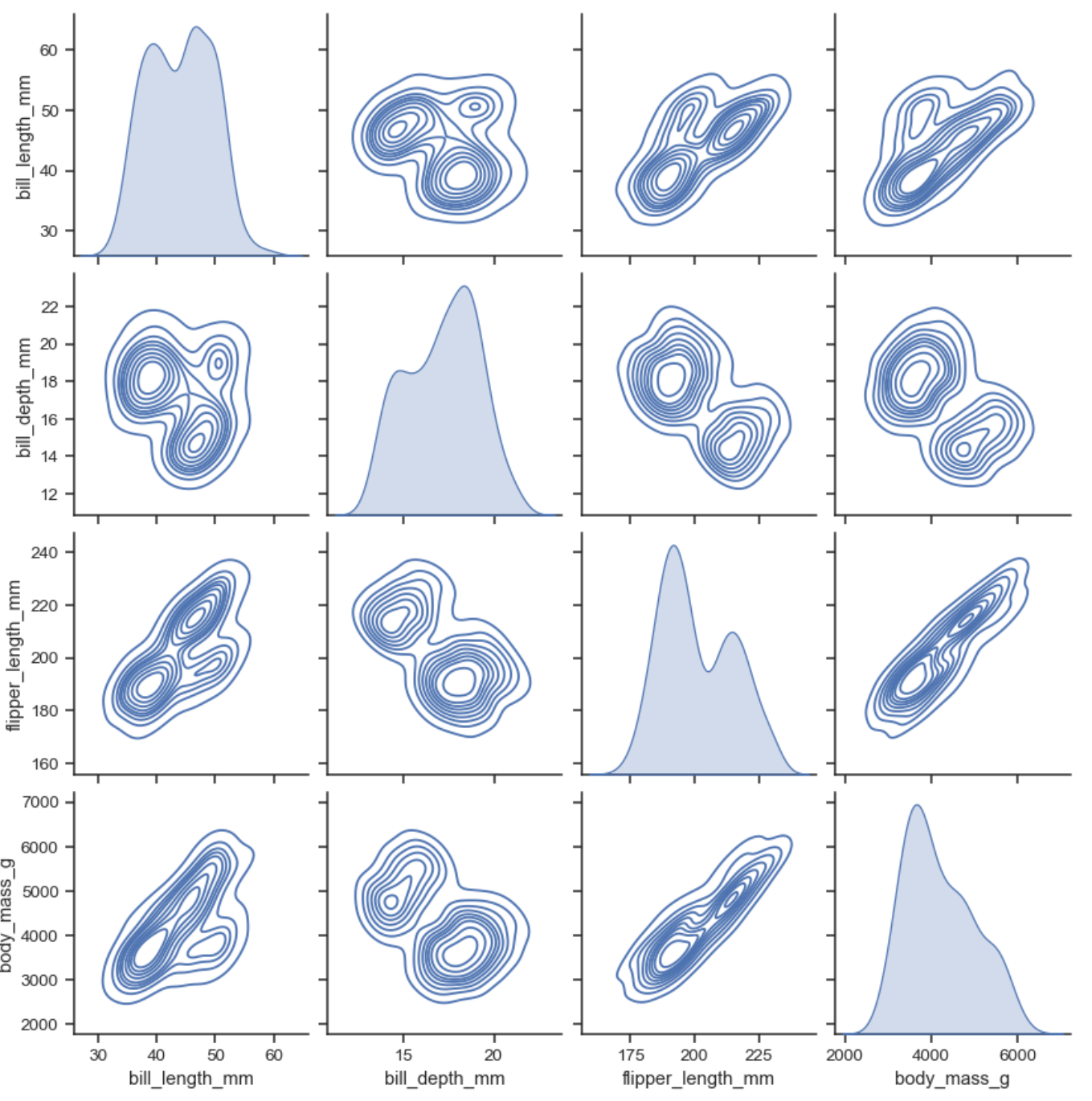
Contour lines on Facet Grid with single KDE line on the diagonal.
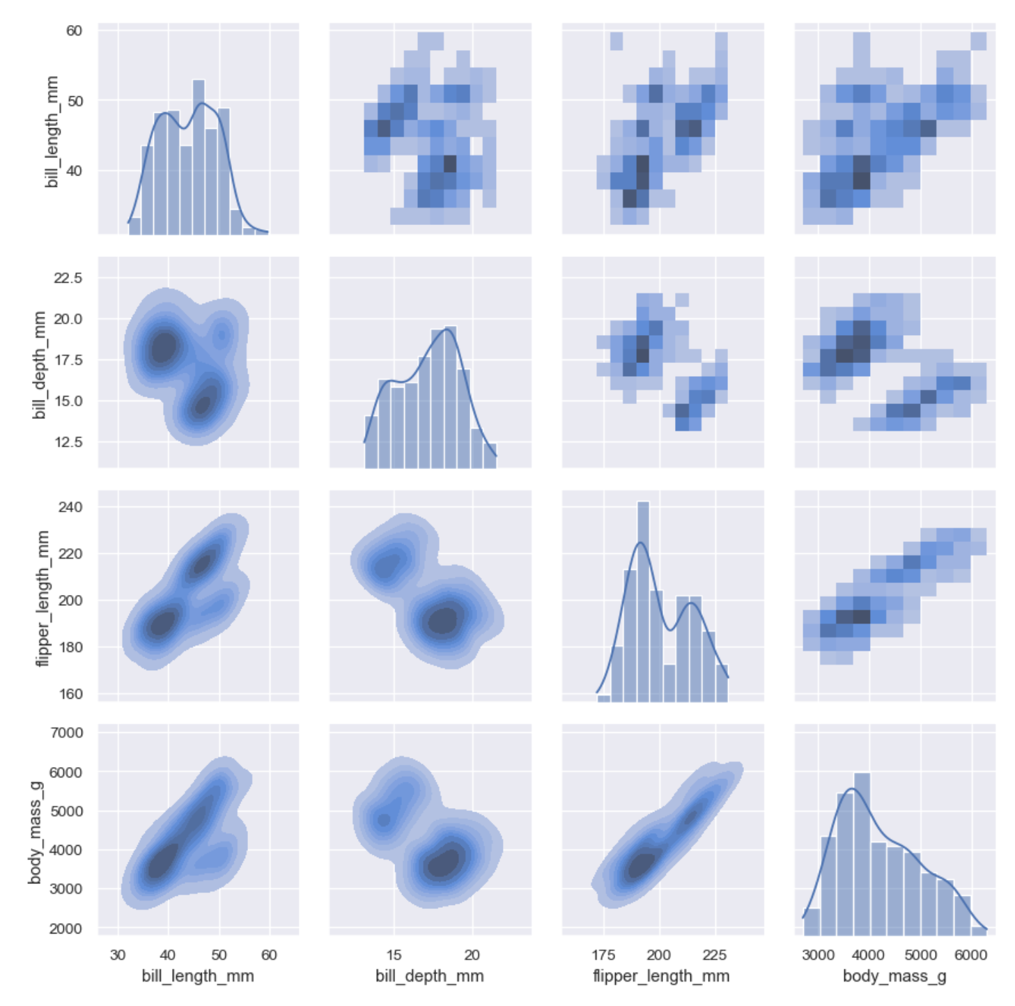
Contour lines on Facet Grid with the histograme of single vector on the diagonal.
Advanced Topics
Kernel Density Estimation (KDE) has several advanced topics that can be explored for a deeper understanding and more effective application. Here are some of these topics:
Adaptive Bandwidth Selection: This involves using different bandwidths for different regions of the data space, based on local density or other data characteristics. It can improve KDE performance for datasets with varying density and complex structures.
Multivariate KDE: Extending KDE to multivariate data involves selecting appropriate kernel functions and bandwidths in multiple dimensions. Handling the curse of dimensionality and the increased computational complexity are important considerations.
Kernel Choice: Different kernel functions can yield different KDE results, and understanding their properties, such as order, continuity, and bias, can guide kernel selection for specific applications.
Density Derivatives: Estimating density derivatives (e.g., gradient, Hessian) using KDE can provide additional insights into the data, such as local maxima and saddle points. This is particularly useful in optimization and feature detection tasks.
Kernel Smoothing in Regression: KDE can be used for nonparametric regression by locally smoothing the data using kernel functions. Nadaraya-Watson and Local Linear Regression are examples of such methods.
Advanced KDE Algorithms: Techniques like Fast Fourier Transform (FFT) or K-D Trees can _speed up] KDE computations for large datasets, while advanced KDE methods like Variable Kernel Density Estimation (VKDE) or Bayesian KDE can handle complex data structures and uncertainty in the density estimates.
Summary
Kernel Density Estimation (KDE) is a non-parametric method to estimate the probability density function of continuous random variables.
KDE works by summing kernel functions centered at each data point, resulting in a smooth density estimate.
Key components of KDE include selecting an appropriate kernel function and bandwidth.
KDE has numerous applications, such as data visualization, outlier detection, and data comparison.
Advanced topics in KDE include adaptive bandwidth selection, multivariate KDE, and handling the curse of dimensionality.