What is Spatial Randomness
The null hypothesis
Spatial Randomness is the absence of any pattern
Spatial Randomness is not interesting
if rejected, then there is evidence of spatial structure---spatially structured
How to interpret Spatial Randomness
the observed spatial pattern is equally likely as any other spatial pattern
no structure
values at one location does not depend on values at other locations/parts of the study area
value at one location does not tell you anything about what might be at the nearby locations
Operationalizing Spatial Randomness
under spatial randomness, the location of values may be altered without affecting the information content of the data
random permutation or reshuffling of values
Actual Distribution. See Luc Anselin’s lecture on Spatial Autocorrelation.
Randomly swapping the values between spatial units---Random Permutation. See Luc Anselin’s lecture on Spatial Autocorrelation.
Random Patterns
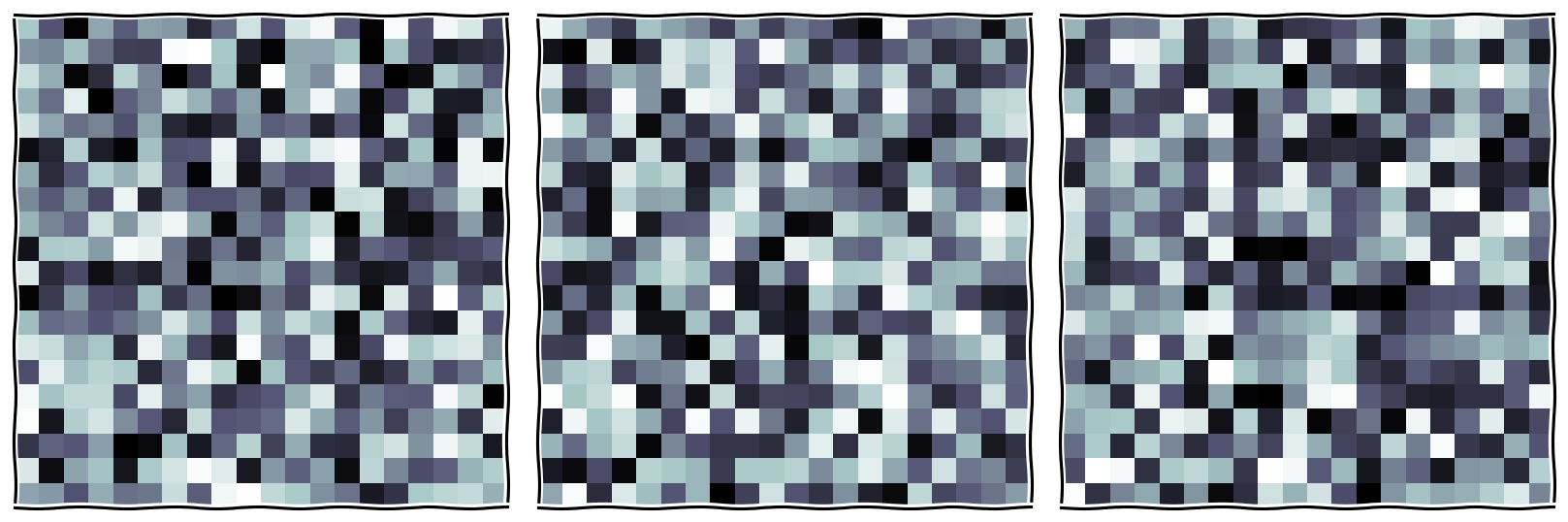
Permutated 3 times. Can you spot the difference?
Tobler’s first law of geography
Everything is related to everything else, but near things are more related than distant things.
Everything depends on everything else, but closer things more so.
Structures spatial dependence
places closer to each other tend to have similar values
values of close locations tend to correlated
the reversed: can we define distance by observing how things are correlated with each other?
if observations are correlated a lot, they are ‘close’
if they are not correlated, they are ‘far’
Importance of distance decay
Distance measure
Spatial adjacency structure
How do you define distance?: Using some distance metrics to ‘structure’ the spatial dependence based on ‘distance decay’ characteristics.
Autocorrelation
The ‘auto-’ in autocorrelation means ‘oneself’. The word ‘autos’ comes from Greek.
Autocorrelation is a measure of the linear relationship between values of a variable and its own nearby values. The ‘self’-correlation here refer to the correlation within one variable itself.
Two common types of autocorrelation:
Temporal: Correlation between values of a variable and its own past or future.
Spatial: Correlation between values of a variable and its own neighbors.
Other types of autocorrelation:
Network: between values of a variable and the connected neighbors.
What is Spatial Autocorrelation
Rejecting the Null Hypothesis: rejecting spatial randomness: the observed spatial pattern is not the result of a random process.
An evidence of Spatial Dependence: values are autocorrelated spatially
An evidence of Spatial Heterogeneity: the underlying probability is non-stationary
Positive Spatial Autocorrelation: similar values in neighboring locations are found to be more frequent compared to spatial randomness
High and High (HH)
Low and Low (LL)
Negative Spatial Autocorrelation: dissimilar values in neighboring locations are found to be more frequent compared to spatial randomness
High and Low (HL)
Low and High (LH)
Spatial Autocorrelation: Global vs. Local
Global Spatial Autocorrelation:
analyzing clustering, compared to spatial randomness
measures the overall degree of spatial clustering or dispersion for the entire study area.
provides a single value (e.g., Moran’s I) that summarizes the extent to which the variable exhibits a clustered, dispersed, or random pattern across the entire area.
the spatial autocorrelation of the entire study area ‘as a whole’
Local Spatial Autocorrelation:
identifying clusters, compared to spatial randomness
calculate the p-value for each location for exploring the probability of becoming a local hot-spot/cold-spot
provides a map (or a series of maps) that shows where the significant hot-spots/cold-spots
use the location-based spatial autocorrelation characteristics to detect posisble clusters at specific locations
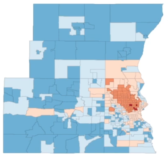
Positive Spatial Autocorrelation
Impression of clustering
Clumps of similar values
‘Similar’ can be both high (hot-spots) or both low (cold-spots)
high values near to each other and
low values near to each other, at the same time
difficult to rely on human perception
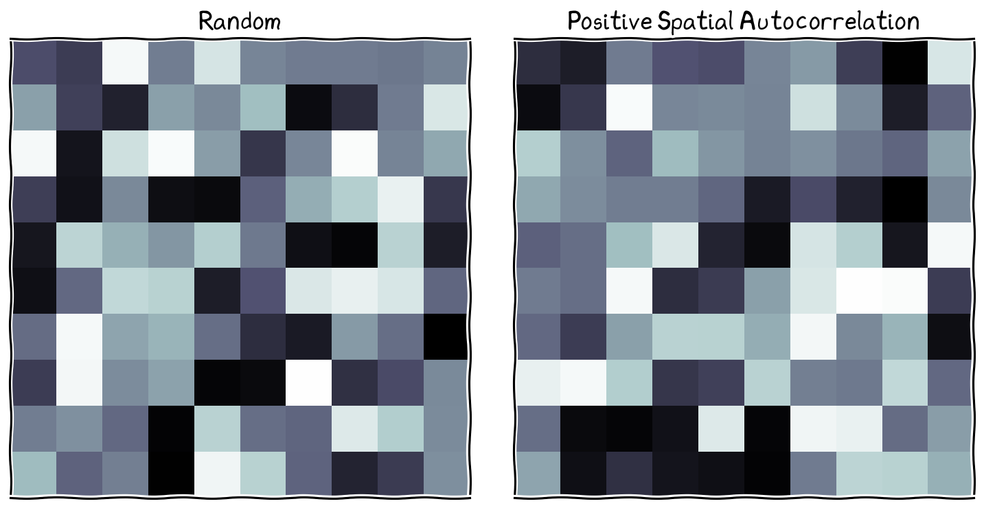
Similar values (either high or low) are closer to each other on the right, compared to the random pattern (left).
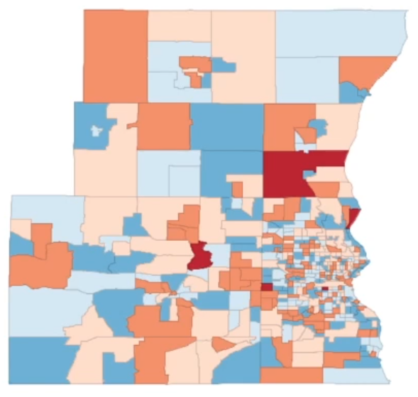
Negative Spatial Autocorrelation
].column[
checkerboard pattern
high value is surrounded by low values
low value is surrounded by high values
alternating values
more about variability
hard to distinguish from spatial randomness
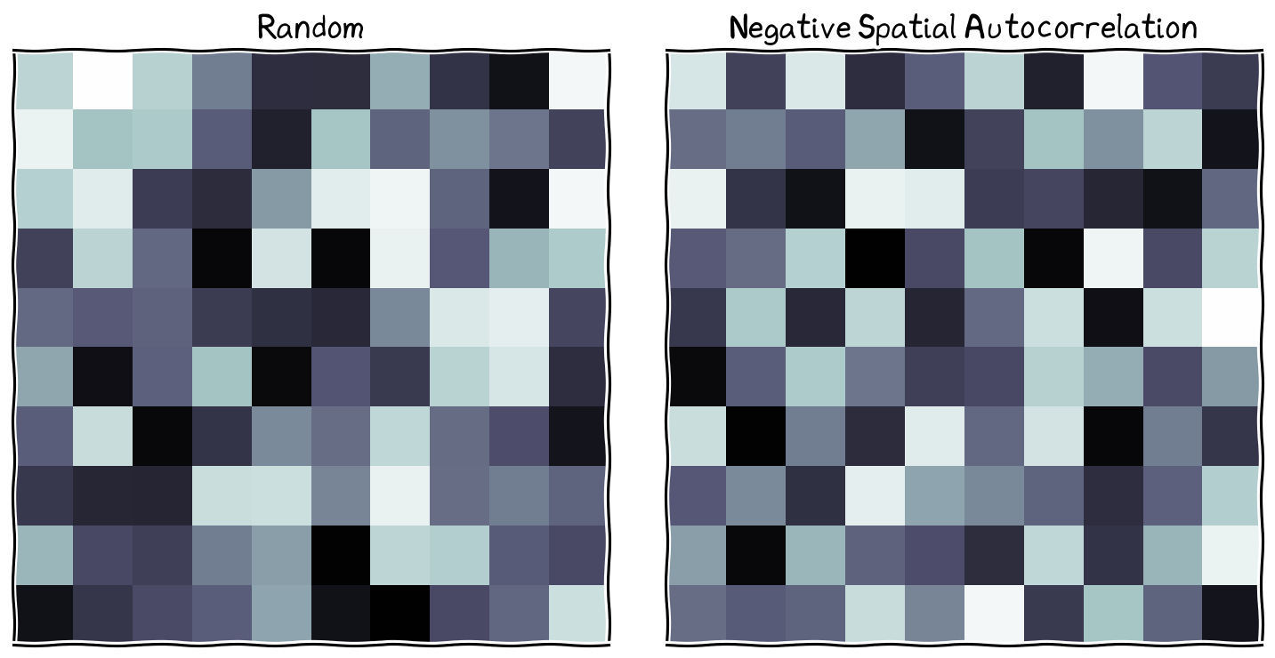
On the right, the dissimilar values are closer to each other, generating checkerboard-like pattern.
Methods for testing Spatial Autocorrelation
There are several statistical methods for testing global spatial autocorrelation, which helps determine whether the observed spatial pattern in a dataset deviates significantly from a random pattern.
Moran’s I: Perhaps the most widely used global spatial autocorrelation measure, Moran’s I statistic evaluates whether the values of a variable are spatially clustered, dispersed, or randomly distributed. Moran’s I ranges from -1 (perfect dispersion) to 1 (perfect clustering), with 0 indicating a random pattern.
Geary’s C: Similar to Moran’s I, Geary’s C measures the degree of spatial autocorrelation in a dataset. While Moran’s I focuses on the correlation between a value and its neighboring values, Geary’s C emphasizes the differences between a value and its neighbors. Geary’s C also ranges from 0 (perfect spatial autocorrelation) to 2 (perfect dispersion), with 1 indicating a random pattern.
Getis-Ord Global G: The Getis-Ord Global G statistic assesses whether the observed spatial pattern exhibits high-value clusters (hotspots) or low-value clusters (coldspots). It provides a single measure of clustering for the entire study area and can be used alongside Moran’s I or Geary’s C to gain additional insights into the data’s spatial structure.
Mantel Test: Originally developed in biology, the Mantel Test is a correlation-based approach that evaluates the relationship between two spatial distance matrices (e.g., geographical and ecological distance matrices). While not strictly a measure of spatial autocorrelation, the Mantel Test can provide valuable insights into the relationship between spatial patterns in different variables.