Defining Distance and neighborhoods - Geospatial Statistics and Visualisation

Adjacency-based spatial weights¶

Spatial relationships based on shared border (a.k.a. rook contiguity). Links on the right show the neighborhood relationship.

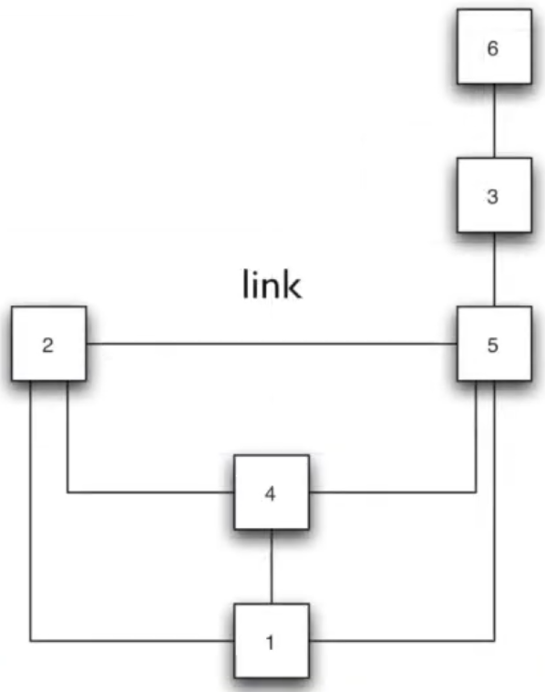
Converting spatial units to nodes and the ‘adjacent relationship’ with links.

Spatial relationships based on shared border (a.k.a. rook contiguity). Links on the left show the neighborhood relationship and the matrix on the right shows the adjacency-matrix / neighborhood matrix.

\text{W} = \begin{bmatrix} 0 & 1 & 0 & 1 & 1 & 0 \\\\ 1 & 0 & 0 & 1 & 1 & 0 \\\\ 0 & 0 & 0 & 0 & 1 & 1 \\\\ 1 & 1 & 0 & 0 & 1 & 0 \\\\ 1 & 1 & 1 & 1 & 0 & 0 \\\\ 0 & 0 & 1 & 0 & 0 & 0 \end{bmatrix}

(1)

Spatial Contiguity¶

A regular grid,
Rook (share edge only)
bishop (share point only)
queen (share edge and point)

Higher levels contiguity can be done by adding second, third, etc. outer ring of neighborhoods.

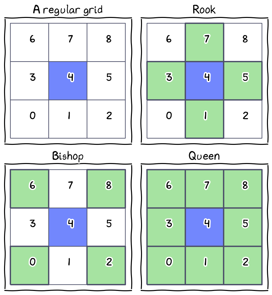
Using the chess concept to define who are the neighbors.

Rook and Queen Contiguity¶

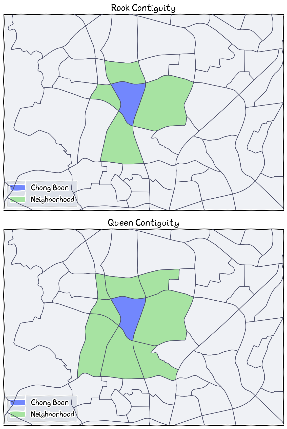
Top: Based on rook contiguity, the Chong Boon Subzone has 4 neighboring subzones. Bottom: Based on queen contiguity, the same Chong Boon Subzone has 8 neighboring subzones (4 additional).

Higher Order Contiguity¶

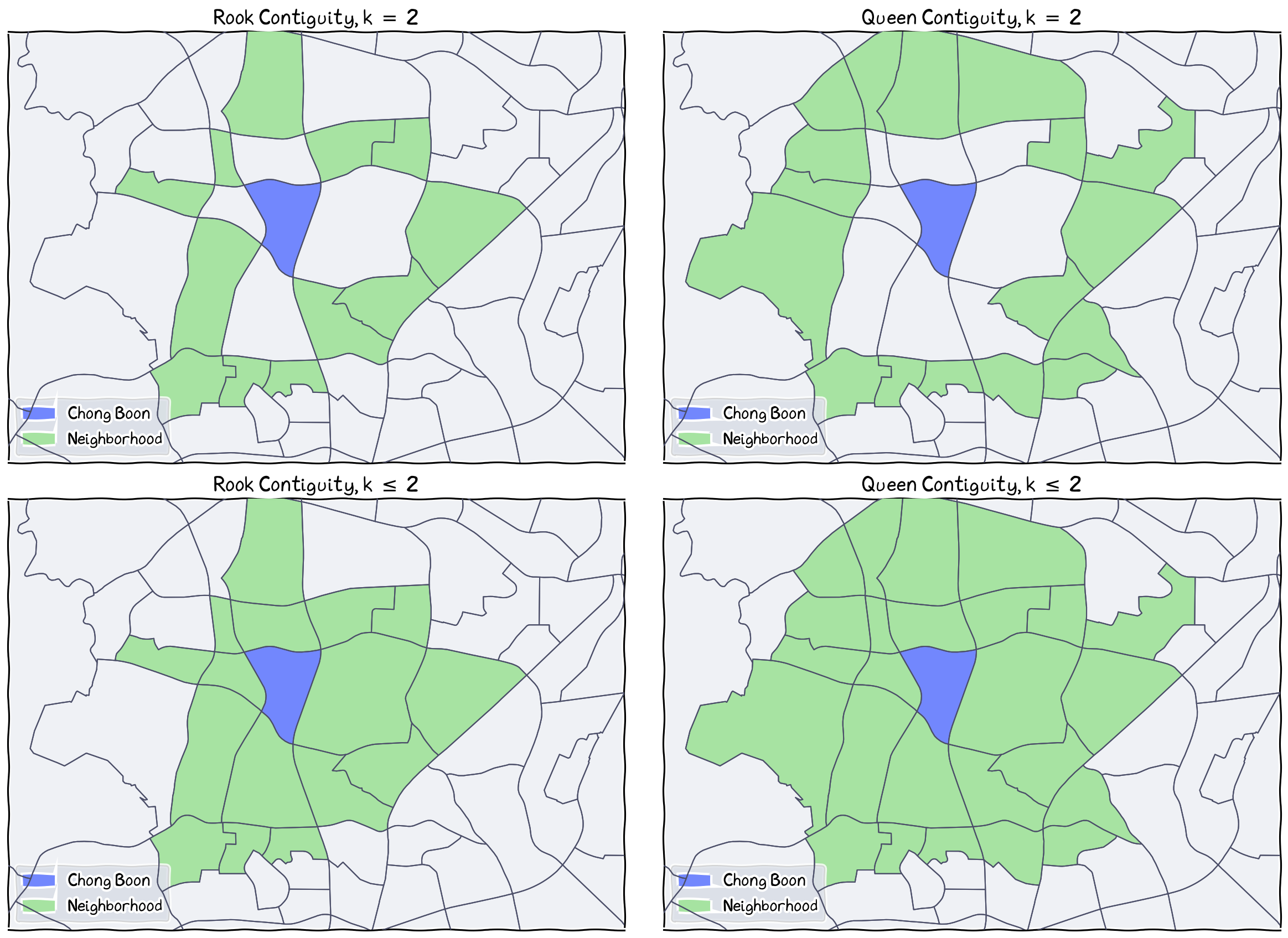
Top: Second level (k=2) contiguity for rook and queen. Bottom: Second level contiguity with lower level (k \leq 2). — Top: Second level (k=2) contiguity for rook and queen. Bottom: Second level contiguity with lower level ( $k \leq 2$ ).

Distance-based Weights¶

a.k.a. distance-band weights
distance between points (polygon centroids, central points)
can be any function of distnace that implies distance decay, e.g., inverse distance
in practice, mostly based on a notion of contiguity defined by distance

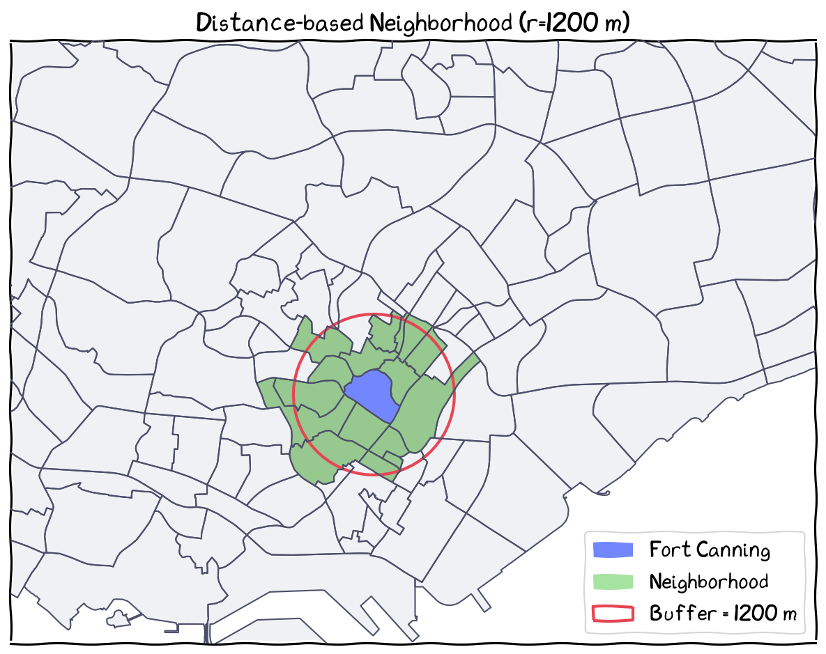
Set a distance band (e.g., 2000 m), draw a buffer as a neighborhood, those spatial units (with their centroid) fall within the buffer are considered neighbors, regardless of the spatial contiguity/adjacency.

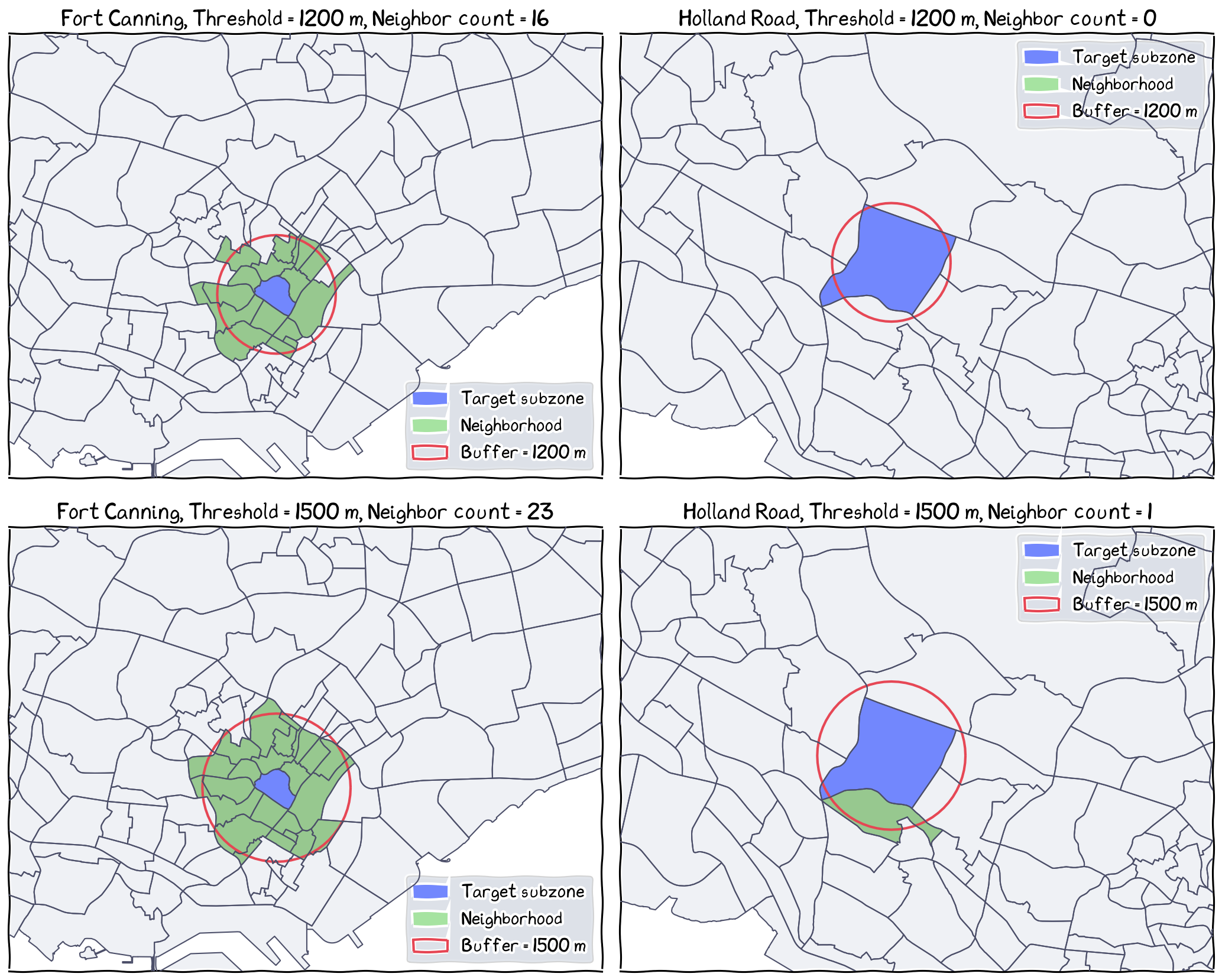
When the size of spatial units vary, the same distance band may generate different numbers of neighbors. E.g., for Fort Canning (left), 1200 m (top) and 1500 m (bottom) distance bands can identify 16 and 23 neighbors, respectively; whereas for Holland Road, the same distance bands can find 0 and 1 neighbor.

k-Nearest Neighbor Weights¶

k-nearest observations, irrespective of distance
- fixed isolates problem for distance bands
- fixed adjacent but not neighbors issue
have the same number of neighbors for all observations
in practice, potential problem with
- ties (observations at the same distance)
- the area size of neighborhood can vary

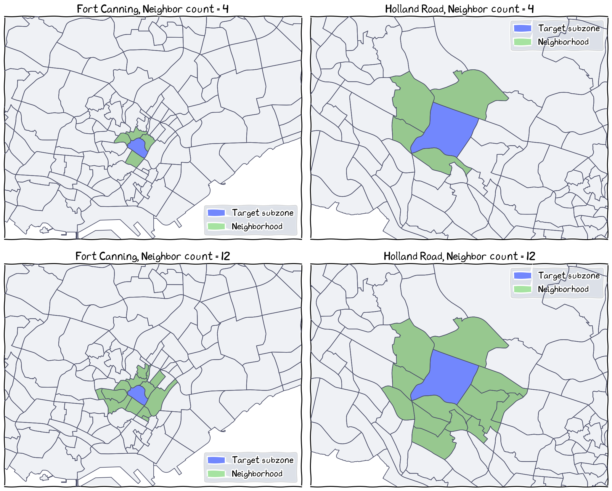
Regardless of variation in distance and spatial contiguity, the k-nearest neighbor approach will sort the neigbors by distance, then select the same number of neighbors (k=4 for top and k=12 bottom). The neighborhood area sizes will be different, depending on the area size of the spatial unit and its nearby units.

Row standardization of Spatial Weights¶

the basic spatial weight uses 1 to indicate neighbors and 0 for non-neighbors
locations with more neighbors with have more ‘1’ in the row (more neighbors) will get more total ‘influences’ by all its neighbors.

\text{W} = \begin{bmatrix} 0 & 1 & 0 & 1 & 1 & 0 \\\\ 1 & 0 & 0 & 1 & 1 & 0 \\\\ 0 & 0 & 0 & 0 & 1 & 1 \\\\ 1 & 1 & 0 & 0 & 1 & 0 \\\\ 1 & 1 & 1 & 1 & 0 & 0 \\\\ 0 & 0 & 1 & 0 & 0 & 0 \end{bmatrix}

(2)

See the last two rows

Row standardization:

is to rescale weights so that for each row i: $\sum(j) w(i,j) = 1$
$w(i,j)' = \frac{w(i,j)}{\sum_k w(i,k)}$
makes calculation results comparable
- all locations will get same level of influence by all their neighbors
- locations with more neighbors, each of its neighbbors will have less weights of influence to the location, such that the total weight of influence from neighbors is the same with any other location
is non-symmetrical.

The original spatial weight matrix:

\text{W} = \begin{bmatrix} 0 & 1 & 0 & 1 & 1 & 0 \\\\ 1 & 0 & 0 & 1 & 1 & 0 \\\\ 0 & 0 & 0 & 0 & 1 & 1 \\\\ 1 & 1 & 0 & 0 & 1 & 0 \\\\ 1 & 1 & 1 & 1 & 0 & 0 \\\\ 0 & 0 & 1 & 0 & 0 & 0 \end{bmatrix}

(3)

Row standardized spatial weight matrix:

\text{W}' = \begin{bmatrix} 0 & 0.333 & 0 & 0.333 & 0.333 & 0 \\\\ 0.333 & 0 & 0 & 0.333 & 0.333 & 0 \\\\ 0 & 0 & 0 & 0 & 0.5 & 0.5 \\\\ 0.333 & 0.333 & 0 & 0 & 0.333 & 0 \\\\ 0.25 & 0.25 & 0.25 & 0.25 & 0 & 0 \\\\ 0 & 0 & 1 & 0 & 0 & 0 \end{bmatrix}

(4)

Geospatial Statistics and Visualisation

Autocorrelation & Spatial Autocorrelation

Geospatial Statistics and Visualisation

Moran’s I