Main goal
Moran’s I is a widely-used measure of global spatial autocorrelation, developed by Australian statistician Patrick Moran. It quantifies the degree to which the values of a variable are spatially correlated with their neighboring values across an entire study area.
Calculation
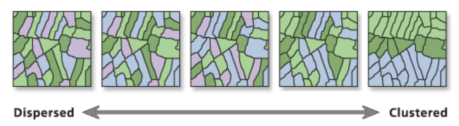
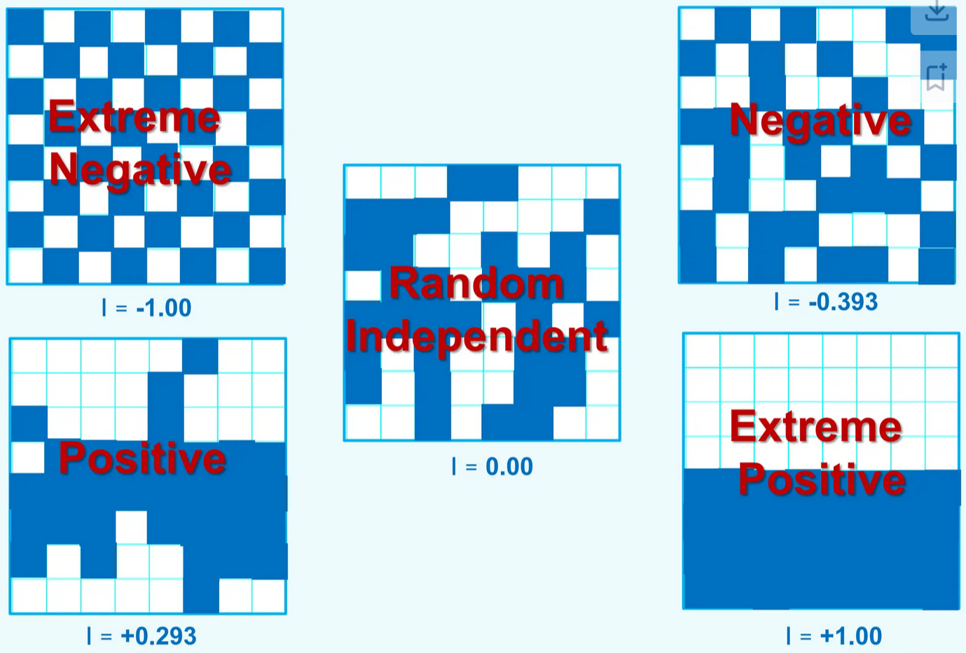
Moran’s I ranges from:
-1 (indicating perfect dispersion or negative spatial autocorrelation) to
+1 (indicating perfect clustering or positive spatial autocorrelation), with
0 indicating a random spatial pattern (no spatial autocorrelation).
Moran’s I is defined as:
Where:
is the number of spatial units indexed by and ;
is the variable of interest;
is the mean of ;
is the spatial weight---kind of an indicator variable, equal to 1 or the row-standardized value if and are neighbors, 0 otherwise;
W is the sum of all .
A significant Moran’s I value suggests that the observed spatial distribution of the variable is not random, and further investigation is warranted to understand the underlying spatial relationships and processes.
Each value is compared to the mean value () before the multiplying. Given the value () of a location and one of its neighbor’s value (), the multiplying result:
is a positive value because both are at the same direction (both higher or both lower);
is a negative value if one of which is higher than the mean and the other is lower compared to mean value;
will be a large value if both the self and neighbor values are very far from the mean value;
will be a small value (near to zero) if the two values are near to mean.
Note that if they are both a lot lower than the mean value, the result would also be a large positive high value, indicating positive spatial Autocorrelation.
Moran’s I: Interpretation
Reading I
theoretical mean is 1/(N-1), essentially zero for large N
positive and significant: clustering of similar value
NOT clustering of high or low
could be either or a combination
negative and significant: alternating values
presence of spatial outliers
spatial heterogeneity (checkerboard pattern)
Comparing the I
Moran’s I depends on spatial weights
relative magnitude for same weights settings and different variables is meaningful
NOT for different spatial weights
use standardized z-value to compare
Moran’s I Scatter Plot
X-axis: the standardized crime rate of every location (town)
Y-axis: the average of standardized neighborhood’s crime rate (spatial-lag of the variable)
Moran’s (written on top)
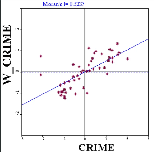
Example of Moran’s scatter plot
The 4 quadrants:
upper right: self-High - lag-High (HH), positively autocorrelated with high values, indicate potential hot-spots;
lower left: self-Low - lag-Low (LL), positively autocorrelated with low values, indicate potential cold-spots;
upper left: self-Low - lag-High (LH), negatively autocorrelated;
lower right: self-High - lag-Low (HL), negatively autocorrelated.
Required statistical testing to identify significant hot-spots and cold-spots.
Permutation Approach
Random reshuffling the attributes data, without modifying the locational data
recompute Moran’s I each time
reconstructing a reference distribution
compare the (original data) observed value of Moran’s I to the reference distribution
even a high Moran’s I value does not necessarily indicate significance.
the ‘p-value’ is not the same as the statistical p-value, it should be called pseudo-p-value as it is calculated using a permutation approach from empirical data, rather than estimated with some solid statistical method.
the number of permutation will ‘improve’ the p-value.
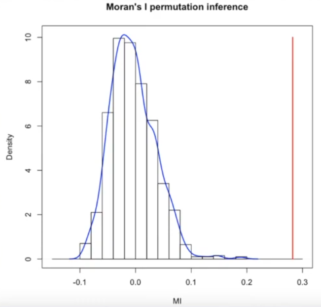
A demo of the permutation distribution. The observed value (orange vertical line) is far higher than the distribution derived from the random permutations.
A demonstration
Moran’s Scatter plot
The bus ridership aggregated by incoming flow, during the morning peak (7am-9am) in June 2023. Spatial weights are 2 levels of Queen contiguity.
The Moran’s I result: 0.03
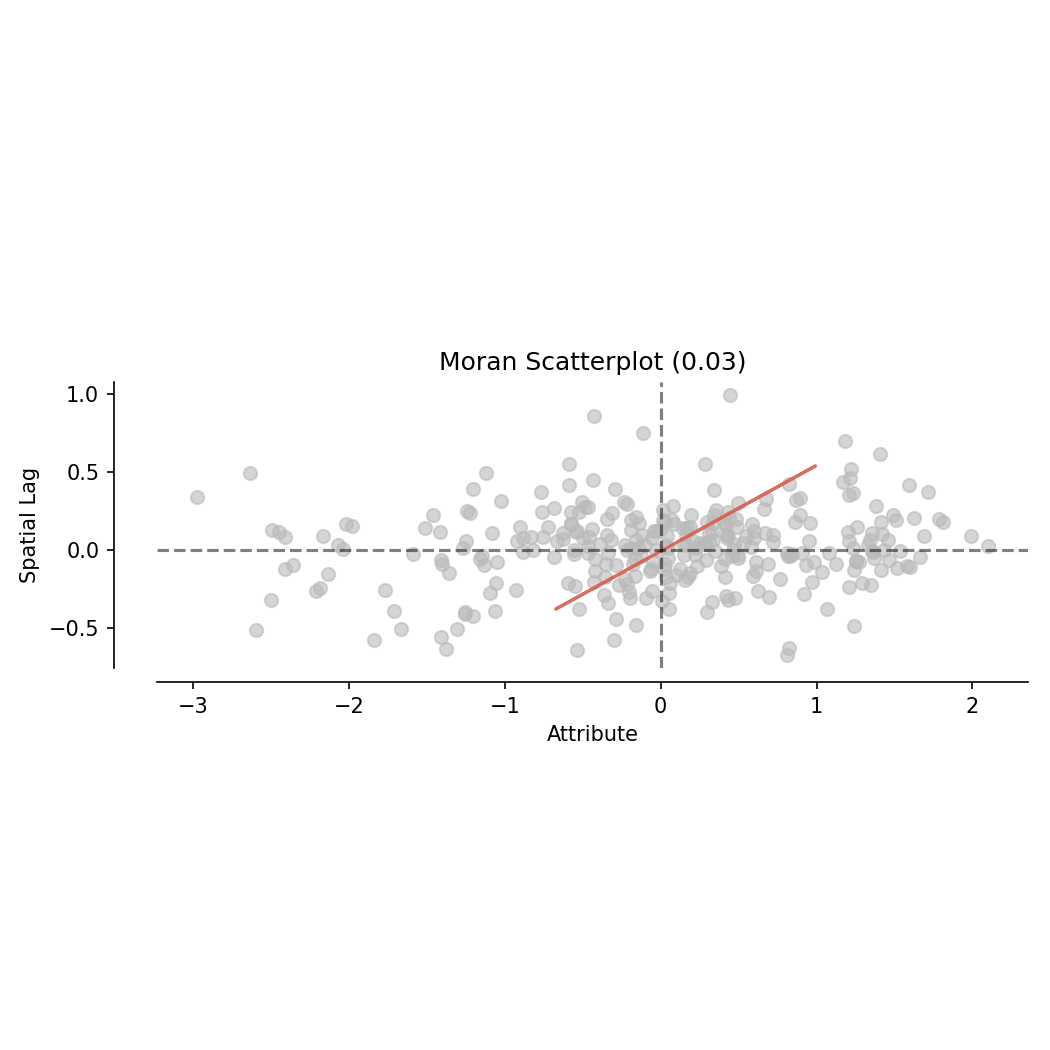
Moran’s I scatter plot of the bus ridership
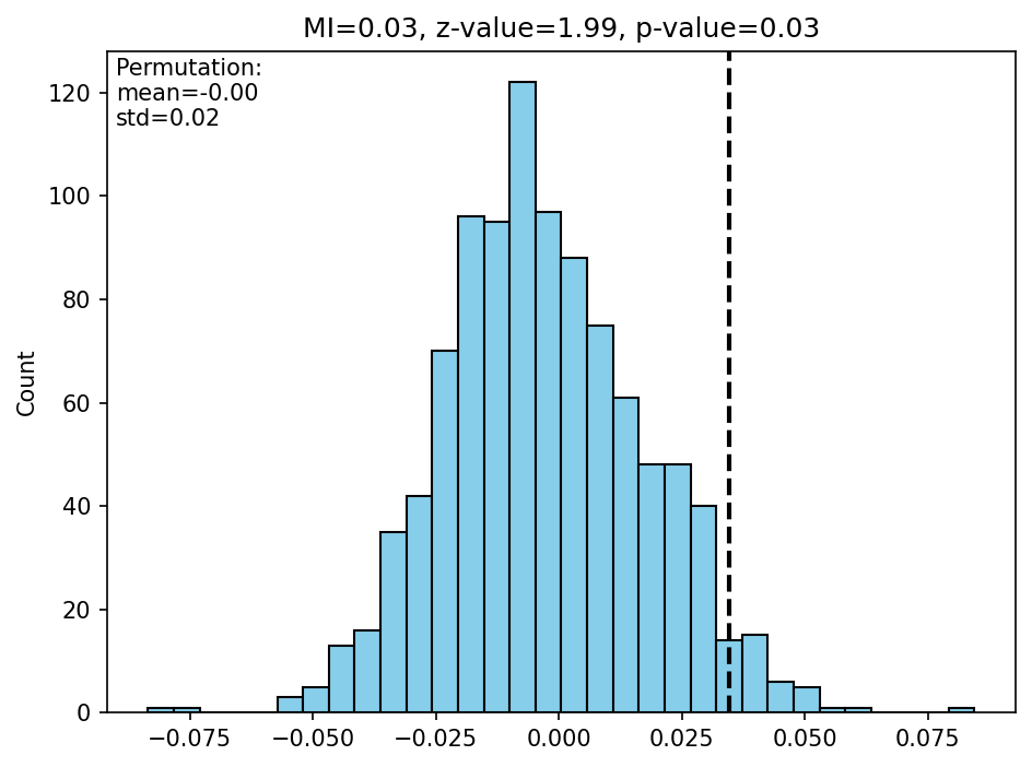
999 times permutation is generated. The observed value (vertical dash line) is somewhere at a higher value range of the distribution.
Closing Remarks
spatial randomness for areal data
spatial autocorrelation
spatial dependency and spatial heterogeneity
attributes similarity and locational similarity
spatial weights and row standardization
contiguity (rook, queen) and higher order
distance-based
k-nearest neighbors
Moran’s I
goals to identify positive and negative spatial autocorrelation
calculation
how to read the result
permutation