What is LISA
LISA, which stands for Local Indicators of Spatial Association, is a set of statistical measures used in spatial data analysis to identify and assess local patterns of spatial autocorrelation. LISA helps detect areas with significant concentrations or disparities of a given variable, such as regions with high crime rates, low-income neighborhoods, or areas with a high prevalence of a particular disease.
LISA encompasses various types of measures, including Local Moran’s I, Local Geary’s C, Gi, and Gi*. These measures build upon the concept of global spatial autocorrelation, measured by Moran’s I (for Local Moran), Geary’s C (for local Geary C), by providing location-specific insights into spatial structures, mainly on spatial clustering (hot-spots, cold-spots) and spatial outliers (neighboring with the opposite type).
By analyzing the spatial patterns and local clustering of a given variable through the different LISA measures, researchers can gain valuable insights for urban planning, public health, environmental studies, criminology, and other fields where spatial relationships and interactions play a crucial role.
LISA form of global spatial autocorrelation
Decomposable statistics
then
What is Local Moran’s
Local Moran’s I is a measure of spatial autocorrelation used in geography and geographic information science (GIS) to assess the degree of spatial clustering or dispersion of a given variable around a specific location. Developed by Anselin (1995), it is a local version of the global Moran’s I statistic, which measures the overall spatial autocorrelation in a dataset.
Local Moran’s I helps identify the extent of significant spatial clustering of similar values around a specific observation. It calculates the correlation between a value at a given location and the values at neighboring locations, highlighting areas with high or low concentrations of the variable under study. This information can be useful in various applications, such as identifying crime hotspots, determining areas with higher disease prevalence, or understanding income disparities across a region.
Essentially, Local Moran’s I provides a way to evaluate spatial patterns and relationships between values at specific locations and their surroundings, offering insights into the spatial structure of the data.
The target of Local Moran
The target of Local Moran is to identify two types of locations with statistical significance (through permutation):
Clusters: locations with significantly similar values (hot-spots & cold-spots)
Outliers: locations with significantly different values.
Places with very similar but not far from the means are ignored (as non-significant).
Clusters: To identify locations with positive correlation:
High-High (HH) clusters: high value locations surrounded by high value neighbors
Low-Low (LL) clusters: low value locations surrounded by low value neighbors
Outliers: To identify locations with negative correlation:
High-Low (HL) outliers: high value locations surrounded by low value neighbors
Low-High (LH) outliers: low value locations surrounded by high value neighbors
Global Moran’s I: Formula
The lower part (denominator) is a kind of standardizig process to control the range of the resulting values.
Where:
is the number of spatial units indexed by and ;
is the variable of interest;
is the mean of ;
is the spatial weight---kind of an indicator variable, equal to 1 or the row-standardized value if and are neighbors, 0 otherwise;
W is the sum of all .
Let’s (i.e., deviations from mean), then
Local Moran’s I: Formula
The lower part (denominator, ) is a kind of standardizig process to control the range of the resulting values.
rearrange...
will not change with , thus constant and this could be captured by the form of:
Technical aspects of Local Moran('s I)
The first part ( or ) is a kind of standardizig process to control the range of the resulting values.
for row-standardized weights (such that and cancel out in Moran’s I)
variables as deviations from mean (, positive means greater than mean, and negative means less than mean).
is the deviation from mean for the current location
is the ‘lag’ term, how high or low is the (location ’s) neighbors’ overall value compared to the mean
for non-row-standardised
take note on the ...
Link Local - Global: LISA
take note on the :
or
the global statistics is the average of local statistics
Statistical Inference
analytical and computational
analytical approximation is poor (do not use)
computational approach is based on conditional permutation
Conditional Permutation
Conditional upon value observed at location
hold value at i fixed, random permute remaining n-1 values and recompute local Moran’s I
since leave non-neighbors to be 0, this is same as randomly pick J number of value (without replacement), J is the number of neighbors, then locate these J values on each neighbor for the local Moran calculation.
repeat many times (e.g., 999) to obtain reference distribution for location i, compare and calculate pseudo p-value
computationally intensive:
if there is N size of entity (row), and the permutation is set to 1000, then the calculation takes N * 1000.
Interpretation
Local Significance Map
shows locations with significant local statistic by level of significance.
not very useful for substantive interpretation
useful for observation of the confidence level
diagnostic for sensitivity of results (for example, when only significant at 0.05 but not at 0.001).
An example
Take an example: the donations data (Guerry data)
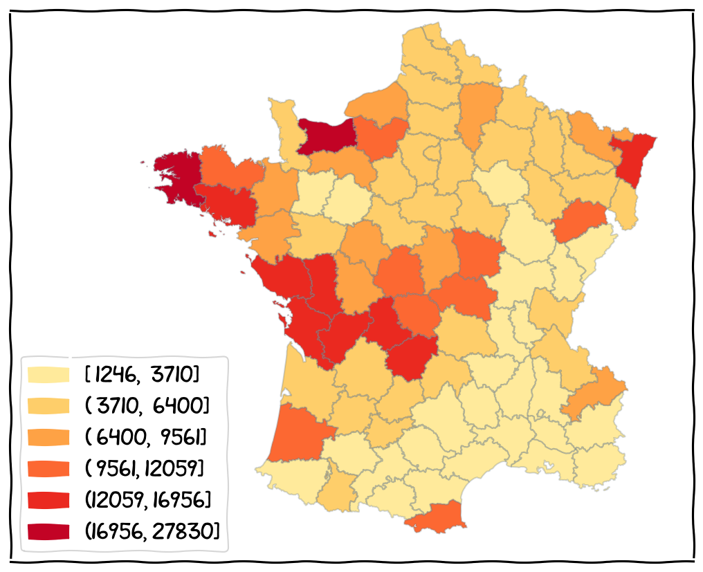
The data distribution (based on Natural Breaks).
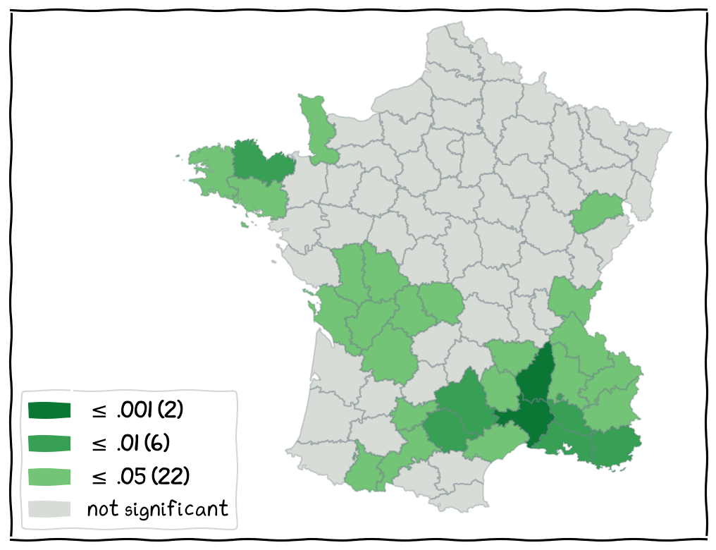
The Local Significance Map
The Local Cluster Map
shows locations with significant local spatial autocorrelation by type of association
four types (four colours):
HH clusters
LL clusters
HL outliers
LH outliers
shown only for a specified significance level (sensitivity analysis)
but the Local Moran can only be used to identify positive or negative correlation, i.e., clusters or outliers, how to differentiate the HH from LL and HL from LH?
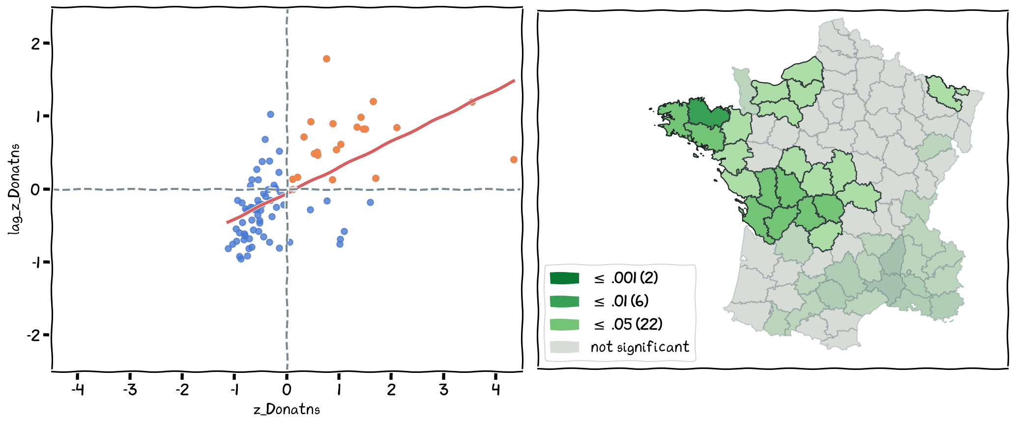
Use the quadrants: For those significant (the map on the right), check the position of the spatial unit in the scatter plot: on top right indicates HH, bottom left LL.
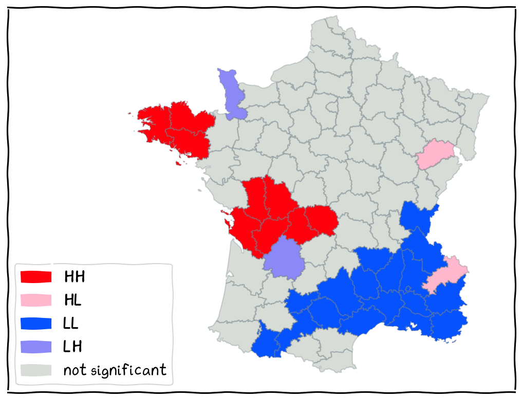
The Local Cluster Map
Sensitivity Analysis Using The Local Cluster Map
Through the changes of significance level, we can observe the changes of clusters/outliers and identify those that is more significant.
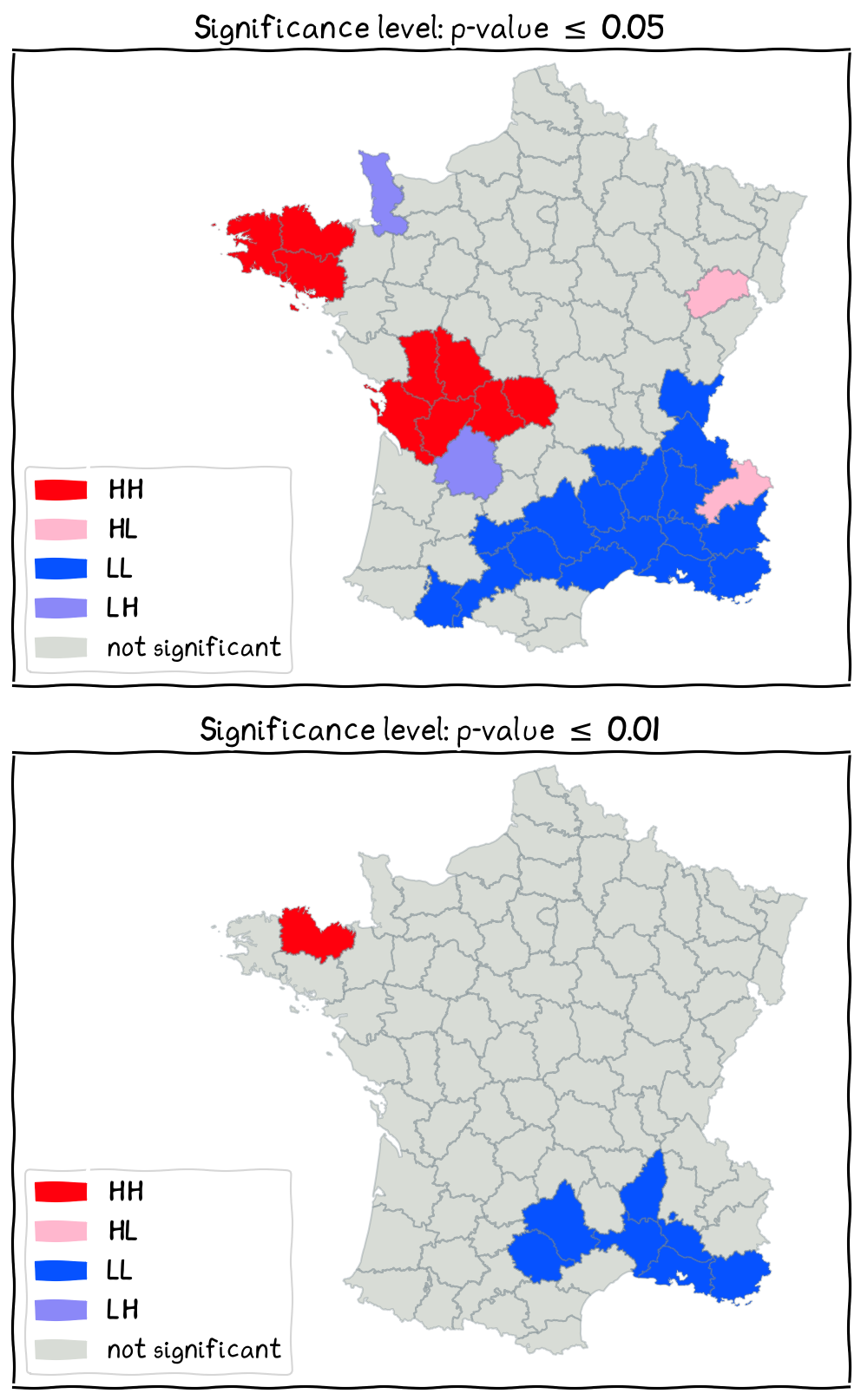
Top: p-value < 0.05; bottom: p-value < 0.01
The Local Outliers
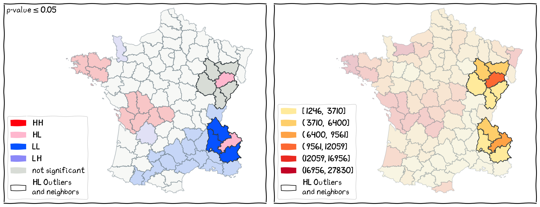
The locations of HL outliers and their neighbors.
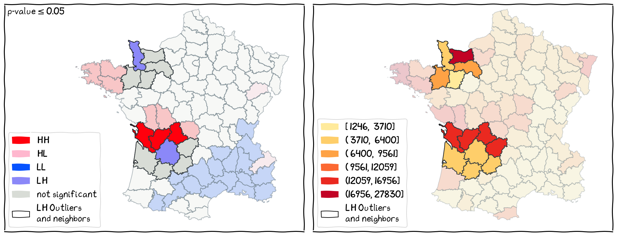
The locations of LH outliers and their neighbors.
The Local Hot-spots
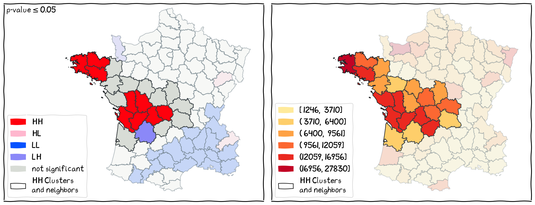
The locations of HH clusters and their neighbors.
The Local Cold-spots

The locations of LL clusters and their neighbors.
Overview
Local Moran’s I is a local measure of spatial autocorrelation used in spatial data analysis. It assesses the degree of spatial clustering or dispersion around individual locations, providing location-specific information about the presence of spatial patterns. As a member of the Local Indicators of Spatial Association (LISA) family, Local Moran’s I builds upon the global Moran’s I statistic to offer a more fine-grained understanding of spatial relationships within a dataset.
Four types of spatial clusters and outliers can be identified:
High-High (HH) clusters (hot-spots),
Low-Low (LL) clusters (cold-spots),
High-Low (HL) outliers, and
Low-High (LH) outliers.
Local Moran’s I results could be observed and discussed in two linked maps, i.e., the local significance map and local cluster map. These maps can be used to visualize the spatial distribution of clusters and outliers, aiding in the interpretation and understanding of spatial patterns.