Geary’s C
Geary’s C is a global measure of spatial autocorrelation used in spatial data analysis to determine the overall degree of spatial dependency in a dataset. It quantifies the degree to which values in a dataset are similar to or different from neighboring values, considering the entire study area. Unlike Moran’s I, Geary’s C focuses on the distance between value of a location and its neighbors rather than their distances to the mean value.
In this equation:
is the number of observations.
is the spatial weight matrix, representing the spatial relationships between observations and .
are the observed values of the variable at location k.
is the sum of all spatial weights.
is the mean of the observed values.
The lower part (denominator) is a kind of standardizig process to control the range of the resulting values.
Local Geary’s C
The Local Geary:
Unlike the global Geary’s C, the local version provides location-specific information about spatial autocorrelation, allowing for the identification of spatial clusters and outliers. Low values of the Local Geary’s C indicate positive spatial autocorrelation (similar values cluster together), while high values indicate negative spatial autocorrelation (dissimilar values are close to each other).
Comparing Global vs. Local
Global
Local
Interpretation
attribute dissimilarity
distance in attribute space
Geary’s C: weighted average of distances in attribute space to neighbors in geographic space
positive: similarity, can be high-high, low-low, middle-middle
negative: dissimilarity: no distinction between high-low and low-high
Geary’s C is more sensitive to local patterns of spatial autocorrelation and can better capture smaller-scale variations in the data. spatial non-stationarity: a sub-region of the study area has a different (e.g., lower) average value, for which the similar-values (could be middle-middle) may be overlooked by Moran’s I (and its local variant).
An example
Take an example: the donations data (Guerry data)
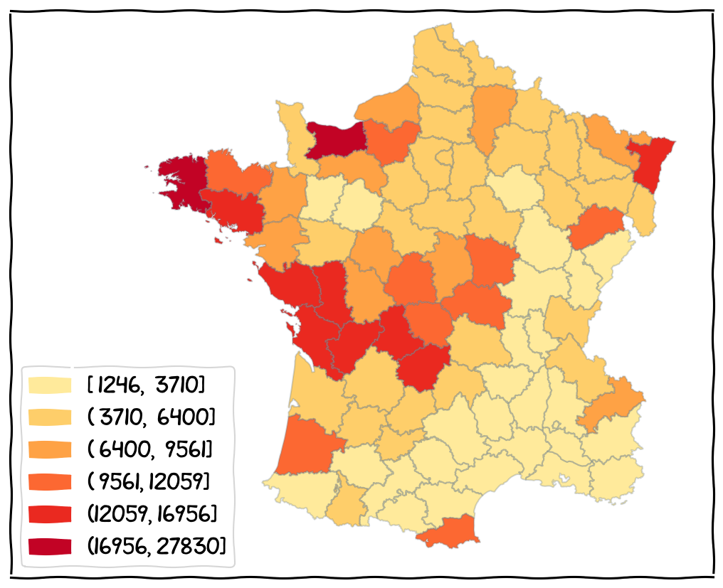
The data distribution (based on Natural Breaks).
Local Significance Map
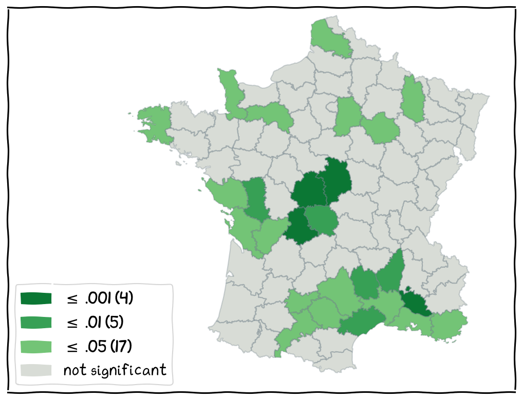
Local Significance Map
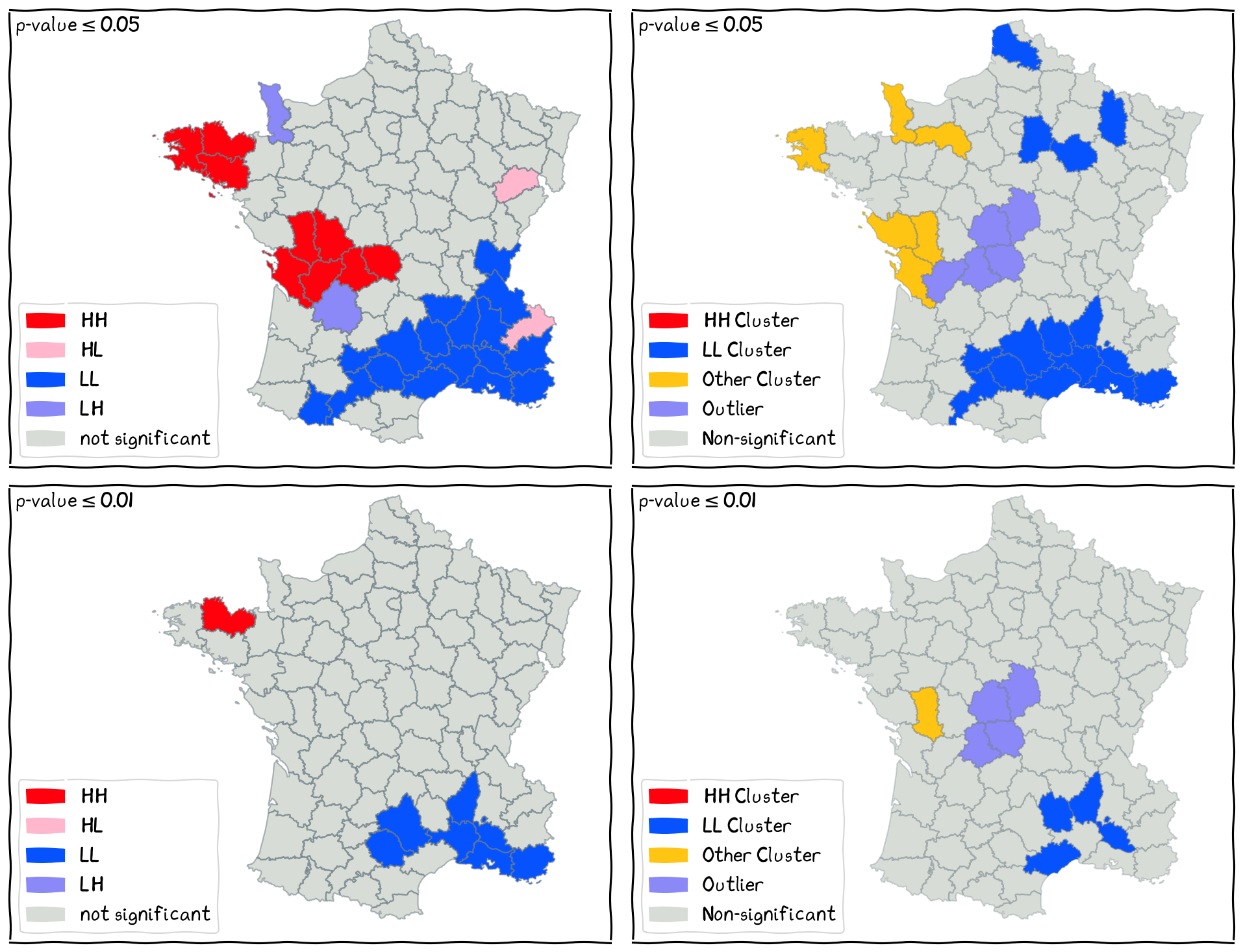
Local Cluster Map
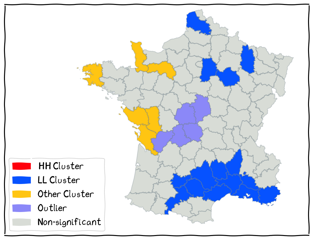
Local Cluster Map
Sensitivity Analysis
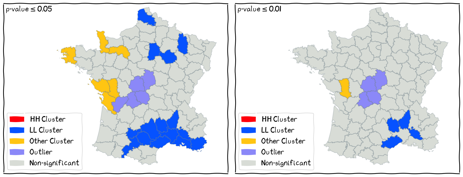
Sensitivity Analysis
Local Moran’s I vs. Local Geary’s C
Comparison between local Moran’s I and local Geary’s C
Moran’s I vs. Geary’s C
Different type of attribute similarity
cross-product (correlation) vs.
squared difference (dissimilarity)
power against different alternatives
the same null hypothesis: spatial randomness
what should be the ‘alternative’?
Moran’s I and its local variant: Detect similar values based on their deviation from the mean value.
Moran’s I is more sensitive to global patterns of spatial autocorrelation and overall trends in the data.
Geary’s C and its local variant: Detect similar values based on the absolute differences between pairs of values.
Geary’s C is more sensitive to local patterns of spatial autocorrelation and smaller-scale variations in the data.