After this page, you should be able to:
Trace how cumulative-cost relaxation improves an earlier route candidate.
Qualify the fastest-route guarantee using the supplied weights and model boundaries.
Builds on: Fewest-link routes, heaps and Dijkstra.
Code languages: Python defines the explanations, figures and self-checks. Use the language guide for native conventions and dependencies. Complete runnable topic examples: Python · JavaScript · Julia.
Reuse the translated graph algorithms and the same invented dataset. Julia travel/build columns are 3 and 4, versus 2 and 3 in Python/JavaScript. The translated construction adjacency is named build_graph_view to distinguish it from the graph-builder function. All versions keep the isolated harbour, distinguish absence from a zero-length route, and separate minutes from construction units.
Accumulate minutes along the route
Now minimise travel minutes from Gate A. The time graph contains positive weights, satisfying Dijkstra’s nonnegative-weight condition. The heap prioritises a tentative whole-route cost, and relaxation can replace an earlier, slower route.
time_distance, time_parent = dijkstra(time_graph, "A")
fastest_route = weighted_path_to("A", "F", time_distance, time_parent)
fastest_minutes = route_total(fastest_route, links, 2)
var [time_distance, time_parent] = dijkstra(time_graph, "A");
var fastest_route = weighted_path_to("A", "F", time_distance, time_parent);
var fastest_minutes = route_total(fastest_route, links, 2);time_distance, time_parent = dijkstra(time_graph, "A")
fastest_route = weighted_path_to("A", "F", time_distance, time_parent)
fastest_minutes = route_total(fastest_route, links, 3)A better route can have more links
After A is processed, B has tentative distance 12 and C has 3. Processing C improves B to 5 via A–C–B, proposes D at 12 and E at 15. Processing B then improves D to 8. D improves E to 11 and proposes F at 16; E finally improves F to 13.
Valid heap pops settle vertices in order A, C, B, D, E, F. The old candidates remain in the lazy heap and are discarded when they no longer match current labels. Final distances are A:0, B:5, C:3, D:8, E:11, F:13; G has infinite distance.
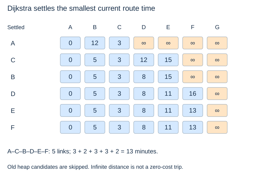
The answer is A–C–B–D–E–F, five links and 13 minutes. Taking more links reduces time in this model. All algorithmic time weights came from column 2; construction cost did not enter the heap key.
Qualify what fastest means
The model adds fixed link times. It excludes waiting, congestion, timetables, fares and transfer penalties. Therefore “least travel time” here means least sum of these supplied weights, rather than a prediction of a real door-to-door journey.
weighted_path_to("A", "G", time_distance, time_parent) returns None, while the source has distance zero. This implementation initialises all declared vertices, unlike BFS’s reached-only distance dictionary. Different containers express different conventions; an absent BFS key and an infinite Dijkstra label both indicate unreachable G here.
Query contract, state and costs
The query returns fresh distance and parent maps for every declared place without changing the graph. It requires a declared source, valid endpoints and finite nonnegative weights; this case supplies positive weights. The implementation explicitly rejects an unknown source with KeyError and a negative weight with ValueError. That negative-weight scan covers the whole graph, including unreachable components. It is not full validation of malformed records or non-finite numbers.
Each finite tentative label is the cost of a discovered route. Relaxation keeps a better label and matching predecessor; an obsolete heap entry is skipped. At a valid minimum-cost pop, nonnegative remaining edges prevent an undiscovered cheaper completion to that vertex. This is the settlement argument; discovery alone is insufficient.
weighted_path_to assumes distance and parent maps from the same run and the matching source. It returns ["A"] for A, None for infinite-distance G, and raises KeyError for an unknown target because it indexes distance[target]. Its source argument does not validate the maps. Keep the source and both maps together when reusing results.
With n vertices and m undirected links, the shown lazy-heap version takes O(n+m log(m+2)) time and O(n+m) auxiliary/result storage. Initialisation and weight validation are included; stale candidates can occupy more than one heap slot per vertex. Recovering a k-edge route adds O(k+1) time/output, and measuring it adds the adapter cost. Reuse all-source-A distances for several destinations until weights or links change.
Check your understanding
Predict the result or justify the choice before opening the explanation.
1. May B be marked final when A first proposes its cost as 12?
Show explanation
No. Processing C later discovers A–C–B at cost 5. B becomes settled at its valid minimum-cost pop, not at first insertion.
2. After adding a five-minute boarding wait at every intermediate stop, can we still report 13 minutes as the optimum journey time?
Show explanation
No. The supplied weights omitted those waits. The current route has four intermediate stops and would total 33 minutes under that rule; other routes must be compared again using a model that includes the new costs.
Next: Incremental connectivity.