After this page, you should be able to:
Explain why merging sorted halves establishes the whole sorting contract.
Relate slicing, left-first ties and temporary lists to time, space and stability.
Builds on: Recursion and the sorting contract. The divide-and-conquer reading develops the same implementation from recursive calls.
Code languages: Python defines the explanations, figures and self-checks. Use the language guide for native conventions and dependencies. Complete runnable topic examples: Python · JavaScript · Julia.
Teaching sorts retain their mutation/return policy: JavaScript mutators return undefined and Julia teaching mutators return nothing. Built-in sort APIs are shown separately: JavaScript sort and Julia sort! return their mutated arrays. The Timsort/Powersort discussion describes Python’s implementation, not the algorithms used by the other runtimes.
Idea and visual trace
Split by position until each part has at most one item, then merge sorted results. The split does not classify values around a pivot: both halves can contain small and large keys.
For the shared sorting input [7,2,6,3,5], the top-level halves are [7,2] and [6,3,5]. Recursive sorting returns [2,7] and [3,5,6]. Comparing their first unused values emits 2,3,5,6, then the remaining 7.
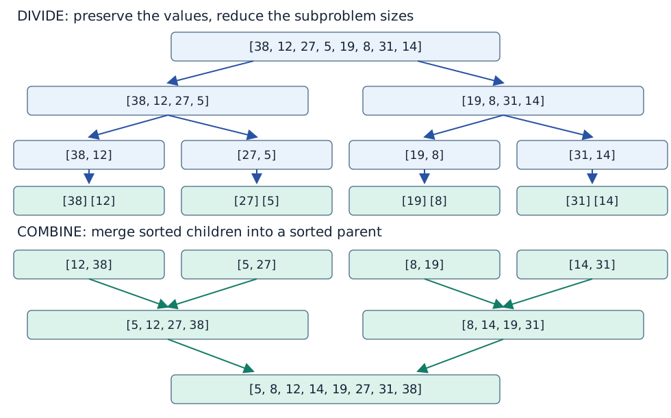
The figure uses the eight-value example from Topic 3 to show all levels. The five-value trace above applies the same rule; odd lengths simply produce halves differing by one item.
Python implementation
This is the same code as Topic 3. It returns a new list and preserves the caller’s list. It accepts mutually comparable values; there is no key or reverse parameter in this teaching version.
def merge_sorted(left, right):
    result = []
    i = j = 0
    while i < len(left) and j < len(right):
        if left[i] <= right[j]:
            result.append(left[i])
            i += 1
        else:
            result.append(right[j])
            j += 1
    result.extend(left[i:])
    result.extend(right[j:])
    return result

def merge_sort(values):
    if len(values) <= 1:
        return values.copy()
    middle = len(values) // 2
    left = merge_sort(values[:middle])
    right = merge_sort(values[middle:])
    return merge_sorted(left, right)
function merge_sorted(left, right) {
const result = [];
let i = 0, j = 0;
while (i < left.length && j < right.length) {
if (left[i] <= right[j]) result.push(left[i++]);
else result.push(right[j++]);
}
while (i < left.length) result.push(left[i++]);
while (j < right.length) result.push(right[j++]);
return result;
}
function merge_sort(values) {
if (values.length <= 1) return values.slice();
const middle = Math.floor(values.length / 2);
return merge_sorted(merge_sort(values.slice(0, middle)), merge_sort(values.slice(middle)));
}function merge_sorted(left, right)
result = Any[]
i, j = 1, 1
while i <= length(left) && j <= length(right)
if left[i] <= right[j]
push!(result, left[i]); i += 1
else
push!(result, right[j]); j += 1
end
end
append!(result, left[i:end])
append!(result, right[j:end])
return result
end
function merge_sort(values)
length(values) <= 1 && return copy(values)
middle = div(length(values), 2)
return merge_sorted(merge_sort(values[1:middle]), merge_sort(values[middle+1:end]))
endWhy it works
Empty and singleton inputs are sorted. For larger inputs, both recursive problems are strictly smaller. Assume their results are sorted permutations of their inputs. During merging, the smallest unused item must be at one of the two fronts; selecting it maintains an ordered output prefix without losing a record. Once one side is exhausted, the other’s sorted remainder can be appended. This proves order, multiplicity preservation and termination together.
Implementation choices
| Choice here | Consequence or alternative |
|---|---|
| Split with list slices | Allocates shallow lists of references; does not deeply copy records |
| Index into each sorted half | Avoids repeated pop(0), which shifts the remaining Python-list entries |
| Append into a fresh result | Makes the merge easy to trace; requires temporary storage |
| Recurse before merging | Top-down strategy; bottom-up merging can instead use loops over run sizes |
| No already-ordered shortcut | Even sorted input follows the full split/merge pattern |
An index-range implementation with a reusable buffer can reduce allocation overhead while retaining O(n) auxiliary space. These alternatives change implementation costs; they do not change the sorting contract.
Stability and in-place behaviour
Left-first <= ties preserve the order of equal-key records. Each recursive half is stable, and an equal record from the earlier half stays before one from the later half. Choosing the right record first on equality would break that guarantee.
This version is stable and not in place: it returns a new list and uses growing temporary lists. The result shares its payload objects with the input; sorting is not a deep-copy operation.
Time and space costs
Under constant-time comparisons, each level performs linear total slicing/merging work and there are logarithmically many levels. For n≥2, best, average and worst time are Θ(n log n) for this version. Empty and singleton inputs take constant time. There is no random-input assumption needed for the worst-case bound.
Peak additional live storage is O(n), including temporary lists, returned output and the O(log n) call stack. The total number of references allocated/copied over the execution can be Θ(n log n); that cumulative work is different from peak live storage. See implementation costs.
When to use it
Use this algorithm to understand stable divide-and-conquer sorting and predictable worst-case growth. It is useful when extra array storage is acceptable. For practical Python sorting, use the built-in interfaces discussed with Timsort.
Check your understanding
1. With fronts 7 and 3, which item is emitted next? Can 7 be discarded?
Show explanation
Emit 3 and advance only that side. Keep 7 for a later comparison or the remainder; discarding it would violate record preservation.
2. If equal-key records 4_A and 4_B lie in the left and right halves respectively, which must be selected first for stability?
Show explanation
4_A. It came earlier in the original list, and the left-first tie rule preserves that order.
Next: Partitioning, the building block for quicksort.